
Speed Dating Experiment
Valentine's day is fast approaching and those who are in a relationship might start thinking about plans. For those who are not as lucky, read on! Today's guest blogger, Today's guest blogger, Toshi Takeuchi, explores how you can be successful at speed dating events through data.

Contents
- Speed Dating Dataset
- What Participants Looked For In the Opposite Sex
- Were They Able to Find Matches?
- Do You Get More Matches If You Make More Requests?
- Decision to Say Yes for Second Date
- Factors Influencing the Decision
- Validatng the Model with the Holdout Set
- Relative Attractiveness
- Are We Good at Assessing Our Own Attractiveness?
- Attractiveness is in the Eye of the Beholder
- Modesty is the Key to Success
- Summary
Speed Dating Dataset
I recently came across an interesting Kaggle dataset Speed Dating Experiment - What attributes influence the selection of a romantic partner?. I never experienced speed dating, so I got curious.
The data comes from a series of heterosexual speed dating experiements at Columbia University from 2002-2004. In these experiments, you each met all of you opposite-sex participants for four minutes. The number of the first dates varied by the event - on average there were 15, but it could be as few as 5 or as many as 22. Then you were asked if you would like to meet any of them again. You also provided ratings on six attributes about your dates:
- Attractiveness
- Sincerity
- Intelligence
- Fun
- Ambition
- Shared Interests
The dataset also includes participants' preferences on those attributes at various point in the process, along with other demographic information.
opts = detectImportOptions('Speed Dating Data.csv');                % set import options
opts.VariableTypes([9,38,50:end]) = {'double'};                     % treat as double
opts.VariableTypes([35,49]) = {'categorical'};                      % treat as categorical
csv = readtable('Speed Dating Data.csv', opts);                     % import data
csv.tuition = str2double(csv.tuition);                              % convert to double
csv.zipcode = str2double(csv.zipcode);                              % convert to double
csv.income = str2double(csv.income);                                % convert to double
What Participants Looked For In the Opposite Sex
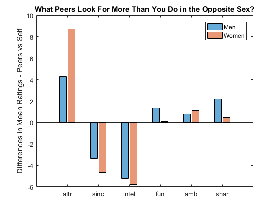
The participants filled out survey questions when they signed up, including what they were looking for in the opposite sex and what they thought others of their own gender looked for. If you take the mean ratings and then subtract the self-rating from the peer rating, you see that participants thought others were more into looks while they were also into sincerity and intelligence. Sounds a bit biased. We will see how they actually made decisions.
vars = csv.Properties.VariableNames;                                % get var names
[G, res] = findgroups(csv(:,{'iid','gender'}));                     % group by id and gender
[~,idx,~] = unique(G);                                              % get unique indices
pref = table2array(csv(idx,contains(vars,'1_1')));                  % subset pref as array
pref(isnan(pref)) = 0;                                              % replace NaN with 0
pref1_1 = pref ./ sum(pref,2) * 100;                                % convert to 100-pt alloc
pref = table2array(csv(idx,contains(vars,'4_1')));                  % subset pref as array
pref(isnan(pref)) = 0;                                              % replace NaN with 0
pref4_1 = pref ./ sum(pref,2) * 100;                                % convert to 100-pt alloc
labels = {'attr','sinc','intel','fun','amb','shar'};                % attributes
figure                                                              % new figure
b = bar([mean(pref4_1(res.gender == 1,:),'omitnan') - ...           % bar plot
    mean(pref1_1(res.gender == 1,:),'omitnan'); ...
    mean(pref4_1(res.gender == 0,:),'omitnan') - ...
    mean(pref1_1(res.gender == 0,:),'omitnan')]');
b(1).FaceColor = [0 .45 .74]; b(2).FaceColor = [.85 .33 .1];        % change face color
b(1).FaceAlpha = 0.6; b(2).FaceAlpha = 0.6;                         % change face alpha
title('What Peers Look For More Than You Do in the Opposite Sex?')  % add title
xticklabels(labels)                                                 % label bars
ylabel('Differences in Mean Ratings - Peers vs Self')               % y axis label
legend('Men','Women')                                               % add legend
Were They Able to Find Matches?
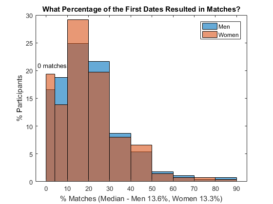
Let's first find out how successful those speed dating events were. If both you and your partner request another date after the first one, then you have a match. What percentage of initial dates resulted in matches?
- Most people found matches - the median match rate was around 13%
- A few people were extremely successful, getting more than an 80% match rate
- About 17-19% of men and women found no matches, unfortunately
- All in all, it looks like these speed dating events delivered the promised results
res.rounds = splitapply(@numel, G, G);                              % # initial dates
res.matched = splitapply(@sum, csv.match, G);                       % # matches
res.matched_r = res.matched ./ res.rounds;                          % match rate
edges = [0 0.4 1:9]./ 10;                                           % bin edges
figure                                                              % new figure
histogram(res.matched_r(res.gender == 1), edges,...                 % histogram of
    'Normalization','probability')                                  % male match rate
hold on                                                             % overlay another plot
histogram(res.matched_r(res.gender == 0), edges,...                 % histogram of
    'Normalization','probability')                                  % female match rate
hold off                                                            % stop overlay
title('What Percentage of the First Dates Resulted in Matches?')    % add title
xlabel(sprintf('%% Matches (Median - Men %.1f%%, Women %.1f%%)', ...% x-axis label
    median(res.matched_r(res.gender == 1))*100, ...                 % median men
    median(res.matched_r(res.gender == 0))*100))                    % median women
xticklabels(string(0:10:90))                                        % use percentage
xlim([-0.05 0.95])                                                  % x-axis range
ylabel('% Participants')                                            % y-axis label
yticklabels(string(0:5:30))                                         % use percentage
legend('Men','Women')                                               % add legend
text(-0.04,0.21,'0 matches')                                        % annotate
Do You Get More Matches If You Make More Requests?
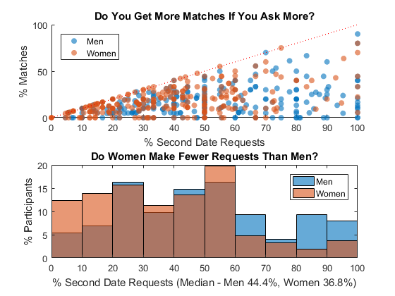
In order to make a match, you need to request another date and get that request accepted. This means some people who got very high match rate must have requested a second date with almost everyone they met and they got their favor returned. Does that mean people who made fewer matches were more picky and didn't request another date as often as those who were more successful? Let's plot the request rate vs. match rate - if they correlate, then we should see a diagonal line!
- You can see some correlation below a 50% request rate - particularly for women. The more requests they make, the more matches they seem to get, to a point
- There is a clear gender gap in request rate - women tend to make fewer requests - the median for men is 44% vs. women for 37%
- If you request everyone, your mileage varies - you may still get no matches. In the end, you only get matches if your requests are accepted
res.requests = splitapply(@sum, csv.dec, G);                        % # requests
res.request_r = res.requests ./ res.rounds;                         % request rate
figure                                                              % new figure
subplot(2,1,1)                                                      % add subplot
scatter(res.request_r(res.gender == 1), ...                         % scatter plot male
    res.matched_r(res.gender == 1),'filled','MarkerFaceAlpha', 0.6)
hold on                                                             % overlay another plot
scatter(res.request_r(res.gender == 0), ...                         % scatter plot female
    res.matched_r(res.gender == 0),'filled','MarkerFaceAlpha', 0.6)
r = refline(1,0); r.Color = 'r';r.LineStyle = ':';                  % reference line
hold off                                                            % stop overlay
title('Do You Get More Matches If You Ask More?')                   % add title
xlabel('% Second Date Requests')                                    % x-axis label
xticklabels(string(0:10:100))                                       % use percentage
ylabel('% Matches')                                                 % y-axis label
yticklabels(string(0:50:100))                                       % use percentage
legend('Men','Women','Location','NorthWest')                        % add legend
subplot(2,1,2)                                                      % add subplot
histogram(res.request_r(res.gender == 1),...                        % histogram of
    'Normalization','probability')                                  % male match rate
hold on                                                             % overlay another plot
histogram(res.request_r(res.gender == 0),...                        % histogram of
    'Normalization','probability')                                  % female match rate
hold off                                                            % stop overlay
title('Do Women Make Fewer Requests Than Men?')                     % add title
xlabel(sprintf('%% Second Date Requests (Median - Men %.1f%%, Women %.1f%%)', ...
    median(res.request_r(res.gender == 1))*100, ...                 % median men
    median(res.request_r(res.gender == 0))*100))                    % median women
xticklabels(string(0:10:100))                                       % use percentage
ylabel('% Participants')                                            % y-axis label
yticklabels(string(0:5:20))                                         % use percentage
legend('Men','Women')                                               % add legend
Decision to Say Yes for Second Date
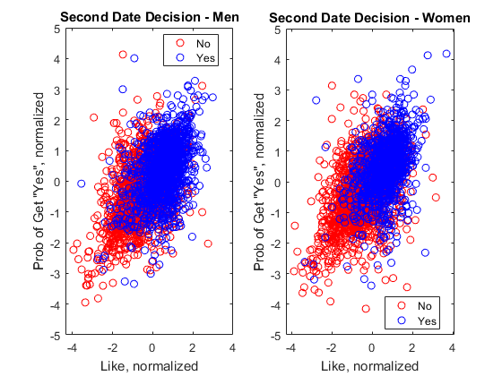
Most people are more selective about who they go out with for second date. The two most obvious factors in such a decision are how much they liked who they met and how likely they think they will get a "yes" from them. There is no point in asking a person for a second date no matter how much you like him or her when you feel there's no chance of getting a yes. You can see a fairly good correlation between Yes and No using those two factors.
Please note that I normalized the ratings for "like" and "probability" (of getting yes) because the actual rating scale differs from person to person. You subtract the mean from the data to center the data around zero and then divide by the standard deviation to normalize the value range.
func = @(x) {(x - mean(x))./std(x)};                                % normalize func
f = csv.like;                                                       % get like
f(isnan(f)) = 0;                                                    % replace NaN with 0
f = splitapply(func, f, G);                                         % normalize by group
like = vertcat(f{:});                                               % add normalized like
f = csv.prob;                                                       % get prob
f(isnan(f)) = 0;                                                    % replace NaN with 0
f = splitapply(func, f, G);                                         % normalize by group
prob = vertcat(f{:});                                               % add normalized prob
figure                                                              % new figure
subplot(1,2,1)                                                      % add subplot
gscatter(like(csv.gender == 1), ...                                 % scatter plot male
    prob(csv.gender == 1),csv.dec(csv.gender == 1),'rb','o')
title('Second Date Decision - Men')                                 % add title
xlabel('Like, normalized')                                          % x-axis label
ylabel('Prob of Get "Yes", normalized')                             % y-axis label
ylim([-5 5])                                                        % y-axis range
legend('No','Yes')                                                  % add legend
subplot(1,2,2)                                                      % add subplot
gscatter(like(csv.gender == 0), ...                                 % scatter plot female
    prob(csv.gender == 0),csv.dec(csv.gender == 0),'rb','o')
title('Second Date Decision - Women')                               % add title
xlabel('Like, normalized')                                          % x-axis label
ylabel('Prob of Get "Yes", normalized')                             % y-axis label
ylim([-5 5])                                                        % y-axis range
legend('No','Yes')                                                  % add legend
Factors Influencing the Decision
If you can correctly guess the probability of getting a yes, that should help a lot. Can we make such a prediction using observable and discoverable factors only?
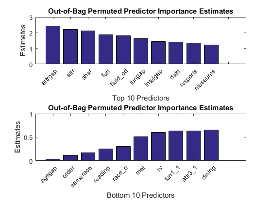
Features were generated using normalization and other techniques - see feature_eng.m for more details. To determine which features matter more, the resulting feature set was then split into training and holdout sets and the training set was used to generate a Random Forest model bt_all.mat using the Classification Learner app. What's nice about a Random Forest is that it can show you the predictor importance estimates based on how error increases if you randomly change the value of particular predictors. If they don't matter, it shouldn't increase the error rate much, right?
Based on those scores, the most important features are:
- attrgap - difference between partners' attractiveness rated by participants and their own self rating
- attr - rating of attractiveness participants gave to their partners
- shar - rating of shared interests participants gave to their partners
- fun - rating of fun participants gave to their partners
- field_cd - participants' field of study
The least important features are:
- agegap - difference between the ages of participants and their partners
- order - in which part of the event they first met - earlier or later
- samerace - whether participants and their partners were the same race
- reading - participant's rating of interest in reading
- race_o - the race of the partners
feature_eng                                                         % engineer features
load bt_all                                                         % load trained model
imp = oobPermutedPredictorImportance(bt_all.ClassificationEnsemble);% get predictor importance
vars = bt_all.ClassificationEnsemble.PredictorNames;                % predictor names
figure                                                              % new figure
subplot(2,1,1)                                                      % add subplot
[~,rank] = sort(imp,'descend');                                     % get ranking
bar(imp(rank(1:10)));                                               % plot top 10
title('Out-of-Bag Permuted Predictor Importance Estimates');        % add title
ylabel('Estimates');                                                % y-axis label
xlabel('Top 10 Predictors');                                        % x-axis label
xticks(1:20);                                                       % set x-axis ticks
xticklabels(vars(rank(1:10)))                                       % label bars
xtickangle(45)                                                      % rotate labels
ax = gca;                                                           % get current axes
ax.TickLabelInterpreter = 'none';                                   % turn off latex
subplot(2,1,2)                                                      % add subplot
[~,rank] = sort(imp);                                               % get ranking
bar(imp(rank(1:10)));                                               % plot bottom 10
title('Out-of-Bag Permuted Predictor Importance Estimates');        % add title
ylabel('Estimates');                                                % y-axis label
xlabel('Bottom 10 Predictors');                                     % x-axis label
xticks(1:10);                                                       % set x-axis ticks
xticklabels(vars(rank(1:10)))                                       % label bars
xtickangle(45)                                                      % rotate labels
ax = gca;                                                           % get current axes
ax.TickLabelInterpreter = 'none';                                   % turn off latex
Validatng the Model with the Holdout Set
To be confident about the predictor values, let's check its predictive perfomance. The model was retained without the bottom 2 predictors - see bt_45.mat and the resulting model can predict the decision of participants to 79.6% accuracy. This looks a lot better than human participants did.
load bt_45                                                          % load trained model
Y = holdout.dec;                                                    % ground truth
X = holdout(:,1:end-1);                                             % predictors
Ypred = bt_45.predictFcn(X);                                        % prediction
c = confusionmat(Y,Ypred);                                          % get confusion matrix
disp(array2table(c, ...                                             % show the matrix as table
    'VariableNames',{'Predicted_No','Predicted_Yes'}, ...
    'RowNames',{'Actual_No','Actual_Yes'}));
accuracy = sum(c(logical(eye(2))))/sum(sum(c))                      % classification accuracy
                  Predicted_No    Predicted_Yes
                  ____________    _____________
    Actual_No     420              66
    Actual_Yes    105             246
accuracy =
       0.7957
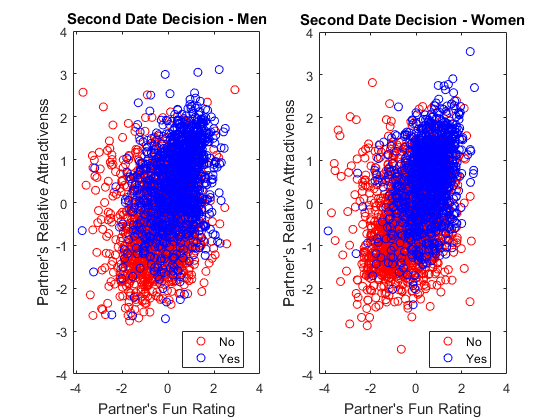
Relative Attractiveness
We saw that relative attractiveness was a major factor in the decision to say yes. attrgap scores indicate how much more attractive the partners were relative to the participants. As you can see, people tend to say yes when their partners are more attractive than themselves regardless of gender.
- This is a dilemma, because if you say yes to people who are more attractive than you are, they are more likely to say no because you are less attractive.
- But if you have some redeeming quality, such as having more shared interests or being fun, then you may be able to get yes from more attractive partners
- This applies to both genders. Is it just me, or does it look like men may be more willing to say yes to less attractive partners while women tends to more more receptive to fun partners? Loren isn't sure - she thinks it's just me.
figure                                                              % new figure
subplot(1,2,1)                                                      % add subplot
gscatter(train.fun(train.gender == '1'), ...                        % scatter male
    train.attrgap(train.gender == '1'),train.dec(train.gender == '1'),'rb','o')
title('Second Date Decision - Men')                                 % add title
xlabel('Partner''s Fun Rating')                                     % x-axis label
ylabel('Partner''s Relative Attractivenss')                         % y-axis label
ylim([-4 4])                                                        % y-axis range
legend('No','Yes')                                                  % add legend
subplot(1,2,2)                                                      % add subplot
gscatter(train.fun(train.gender == '0'), ...                        % scatter female
    train.attrgap(train.gender == '0'),train.dec(train.gender == '0'),'rb','o')
title('Second Date Decision - Women')                               % add title
xlabel('Partner''s Fun Rating')                                     % x-axis label
ylabel('Partner''s Relative Attractivenss')                         % y-axis label
ylim([-4 4])                                                        % y-axis range
legend('No','Yes')                                                  % add legend
Are We Good at Assessing Our Own Attractiveness?
If relative attractiveness is one of the key factors in our decision to say "yes", how good are we at assessing our own attractiveness? Let's compare the self-rating for attractivess to the average ratings participants received. If you subtract the average ratings received from the self rating, you can see how much people overestimate their attractiveness.
- We are generally overestimating our own attractiveness - the median is almost as as much 1 point higher out of 1-10 scale
- Men tend to overestimate more than women
- If you overestimate, then you are more likely to be overconfident about the probability you will get "yes" answers
res.attr_mu = splitapply(@(x) mean(x,'omitnan'), csv.attr_o, G);    % mean attr ratings
[~,idx,~] = unique(G);                                              % get unique indices
res.attr3_1 = csv.attr3_1(idx);                                     % remove duplicates
res.atgap = res.attr3_1 - res.attr_mu;                              % add the rating gaps
figure                                                              % new figure
histogram(res.atgap(res.gender == 1),'Normalization','probability') % histpgram male
hold on                                                             % overlay another plot
histogram(res.atgap(res.gender == 0),'Normalization','probability') % histpgram female
hold off                                                            % stop overlay
title('How Much People Overestimate Their Attractiveness')         % add title
xlabel(['Rating Differences ' ...                                   % x-axis label
    sprintf('(Median - Men %.2f, Women %.2f)', ...
    median(res.atgap(res.gender == 1),'omitnan'), ...
    median(res.atgap(res.gender == 0),'omitnan'))])
ylabel('% Participants')                                            % y-axis label
legend('Men','Women')                                               % add legend

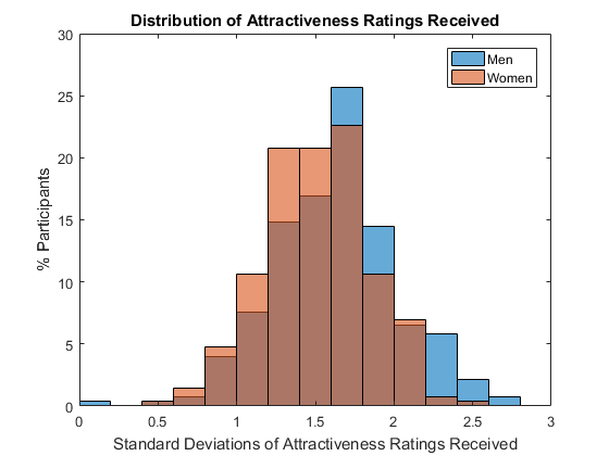
Attractiveness is in the Eye of the Beholder
One possible reason we are not so good at judging our own attractiveness is that for majority of people it it in the eye of the beholder. If you plot to standard deviations of ratings people received, the spread is pretty wide, especially for men.
figure
res.attr_sigma = splitapply(@(x) std(x,'omitnan'), csv.attr_o, G);  % sigma of attr ratings
histogram(res.attr_sigma(res.gender == 1), ...                      % histpgram male
    'Normalization','probability')
hold on                                                             % overlay another plot
histogram(res.attr_sigma(res.gender == 0), ...                      % histpgram female
    'Normalization','probability')
hold off                                                            % stop overlay
title('Distribution of Attractiveness Ratings Received')            % add title
xlabel('Standard Deviations of Attractiveness Ratings Received')    % x-axis label
ylabel('% Participants')                                            % y-axis label
yticklabels(string(0:5:30))                                         % use percentage
legend('Men','Women')                                               % add legend
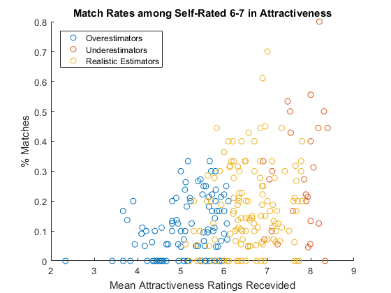
Modesty is the Key to Success
Given that people are not always good at assessing their own attractiveness, how does it affect the ultimate goal - getting matches? Let's focus on average looking people (people who rate themselves 6 or 7) only to level the field and see how the self assessment affects the outcome.
- People who estimated their attractiveness realistically, with the gap from the mean received rating less than 0.9, did reasonably well
- People who overestimated performed the worst
- People who underestimated performed the best
is_realistic = abs(res.atgap) < 0.9;                                % lealitics estimate
is_over = res.atgap >= 0.9;                                         % overestimate
is_under = res.atgap <= -0.9;                                       % underestimate
is_avg = ismember(res.attr3_1,6:7);                                 % avg looking group
figure                                                              % new figure
scatter(res.attr_mu(is_avg & is_over), ...                          % plot overestimate
    res.matched_r(is_avg & is_over))
hold on                                                             % overlay another plot
scatter(res.attr_mu(is_avg & is_under), ...                         % plot underestimate
    res.matched_r(is_avg & is_under))
scatter(res.attr_mu(is_avg & is_realistic), ...                     % plot lealitics
    res.matched_r(is_avg & is_realistic))
hold off                                                            % stop overlay
title('Match Rates among Self-Rated 6-7 in Attractiveness')         % add title
xlabel('Mean Attractiveness Ratings Recevided')                     % x-axis label
ylabel('% Matches')                                                 % y-axis label
legend('Overestimators','Underestimators', ....                     % add legend
    'Realistic Estimators','Location','NorthWest')
Summary
It looks like you can get matches in speed dating as long as you set your expectations appropriately. Here are some of my suggestions.
- Relative attractiveness is more important than people admit, because you are not going to learn a lot about your partners in four minutes.
- But who people find attractive varies a lot.
- You can still do well if you have more shared interests or more fun - so use your four minutes wisely.
- Be modest about your own looks and look for those are also modest about their looks - you will more likely get a match.
We should also remember that the data comes from those who went to Columbia at that time - as indicated by such variables as the field of study - and therefore the findings may not generalize to other situations.
Of course I also totally lack practical experience in speed dating - if you do, please let us know what you think of this analysis compared to your own experience below.
- Category:
- Data Science,
- Fun,
- Machine learning,
- Statistics


Comments
To leave a comment, please click here to sign in to your MathWorks Account or create a new one.