
Surrogate Optimization for Expensive Computations
I'd like to introduce this week's guest blogger Alan Weiss. Alan writes documentation for mathematical toolboxes here at MathWorks.
Hi, folks. This post is about a new solver in Global Optimization Toolbox,
- It is best suited to optimizing expensive functions, meaning functions that are time-consuming to evaluate. Typically, you
use
surrogateopt to optimize a simulation or ODE or other expensive objective function. - It is inherently a global solver. The longer you let it run, the more it searches for a global solution.
- It requires no start point, just problem bounds. Of course, you can specify start points if you like.
The solver is closest in concept to a Statistics and Machine Learning Toolbox™ solver,
Function to Minimize
Let's try to minimize a simple function of two variables:
 ,
,
where  and
and  .
.
x0 = [1,2];
x1 = [-3,-5];
fun = @(x)sum((x/5).^2,2)-4*sech(sum((x-x0).^2,2))-6*sech(sum((x-x1).^2,2));
[X,Y] = meshgrid(linspace(-10,10));
Z = fun([X(:),Y(:)]);
Z = reshape(Z,size(X));
surf(X,Y,Z)
view([53,3])
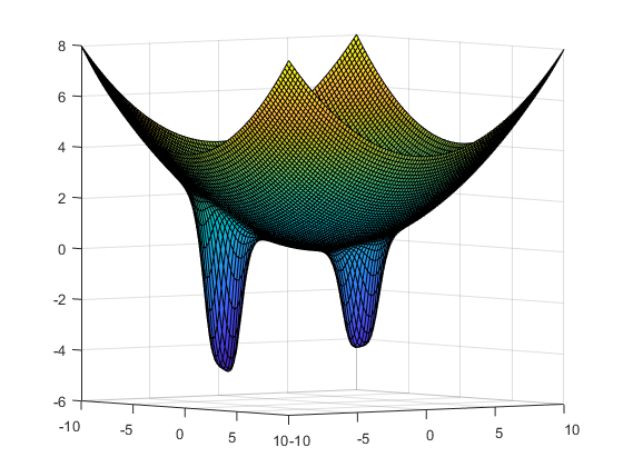
You can see that there are three local minima, the global minimum near [–3,–5], one that is nearly as good near [1,2], and a poor one near [0,0]. You can see this because MATLAB® evaluated 10,000 points for the plot. The value of
Try
surrogateopt
To search for a global minimum, set finite bounds and call
type slowfun
function y = slowfun(x,x0,x1)

y = sum((x/5).^2,2)-4*sech(sum((x-x0).^2,2))-6*sech(sum((x-x1).^2,2));
pause(0.5)
Set bounds and run the optimization of
fun = @(x)slowfun(x,x0,x1);
lb = [-10,-10];
ub = -lb;
rng default % for reproducibility
tic
[xsol,fval] = surrogateopt(fun,lb,ub)
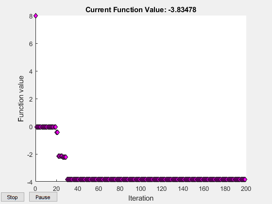
Surrogateopt stopped because it exceeded the function evaluation limit set by
'options.MaxFunctionEvaluations'.
xsol = 1×2

    0.8779    1.7580
fval = -3.8348
toc
Elapsed time is 114.326822 seconds.
Speed Optimization via Parallel Computing
To try to find a better solution, run the solver again. To run faster, set the
options = optimoptions('surrogateopt','UseParallel',true);
tic
[xsol,fval] = surrogateopt(fun,lb,ub,options)
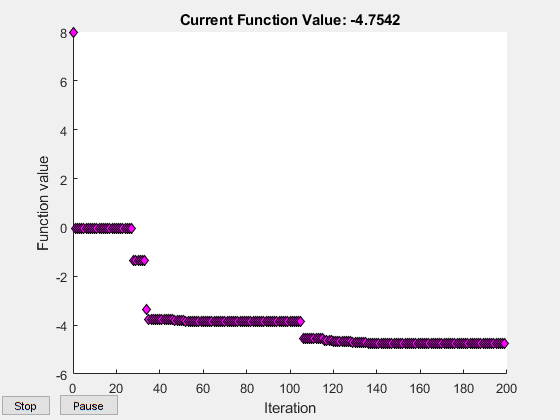
Surrogateopt stopped because it exceeded the function evaluation limit set by
'options.MaxFunctionEvaluations'.
xsol = 1×2

   -2.8278   -4.7159
fval = -4.7542
toc
Elapsed time is 20.130099 seconds.
This time,
How
surrogateopt Works
The
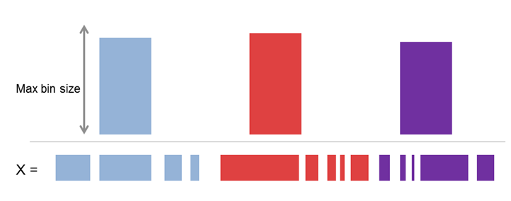
- Construct Surrogate. In this phase, the algorithm takes a fixed number of quasirandom points within the problem bounds and evaluates the objective function at those points. It then interpolates and extrapolates these points to a smooth function called the surrogate in the entire bounded region. In subsequent phases, the surrogate interpolates the evaluated values at all the quasirandom points where the objective has been evaluated. The interpolation function is a radial basis function, because these functions are computationally inexpensive to create and evaluate. Radial basis functions also make it inexpensive to add new points to the surrogate.

- Search for Minimum. This phase is more complicated than the Construct Surrogate phase, and is detailed below.
In theory, there are two main considerations in searching for a minimum of the objective: refining an existing point to get a better value of the objective function, and searching in places that have not yet been evaluated in hopes of finding a better global minimum.
After constructing a merit function,

After evaluating the merit function on the sample points, the solver chooses the point with lowest merit function value, and evaluates the objective function at that point. This point is called an adaptive point. The algorithm updates the surrogate (interpolation) to include this point.
- If the objective function value at the adaptive point is sufficiently lower than the value at the incumbent, then the adaptive point becomes the incumbent. This is termed a successful search.
- If the objective function value at the adaptive point is not sufficiently lower than the value at the incumbent, then the search is termed unsuccessful.
The scale
- If there have been three successful searches since the last scale change, then the scale is doubled:
sigma becomes2*sigma . - If there have been
max(5,nvar) unsuccessful searches since the last scale change, wherenvar is the number of problem dimensions, then the scale is halved:sigma becomessigma/2 .
Generally,
For details, see the Surrogate Optimization Algorithm section in the documentation.
Monitor Optimization Using
surrogateoptplot
You can optionally use the
Run the same problem as before, while using the
options.PlotFcn = 'surrogateoptplot';
options.UseParallel = false;
rng(4) % For reproducibility
[xsol,fval] = surrogateopt(fun,lb,ub,options)

Surrogateopt stopped because it exceeded the function evaluation limit set by
'options.MaxFunctionEvaluations'.
xsol = 1×2

   -2.7998   -4.7109
fval = -4.7532
Here is how to interpret the plot. Starting from the left, follow the green line, which represents the best function value found. The solver reaches the vicinity of the second-best point at around evaluation number 30. Around evaluation number 70, there is a surrogate reset. After this, follow the dark blue incumbent line, which represents the best objective function found since the previous surrogate reset. This line approaches the second-best point after evaluation number 100. There is another surrogate reset before evaluation number 140. Just before evaluation number 160, the solver reaches the vicinity of the global optimum. The solver continues to refine this solution until the end of the evaluations, number 200. Notice that after evaluation number 190, all of the adaptive samples are at or near the global optimum, showing the shrinking scale. There is a similar discussion of interpreting the
Closing Thoughts
I hope that this brief description gives you some understanding of the
Did you enjoy seeing how to use surrogate optimization? Do you have problems that might be addressed by this new solver? Tell us about it here.


Comments
To leave a comment, please click here to sign in to your MathWorks Account or create a new one.