 Cleve’s Corner: Cleve Moler on Mathematics and Computing
 The MATLAB Blog
 Guy on Simulink
 MATLAB Community
 Artificial Intelligence
 Developer Zone
 Stuart’s MATLAB Videos
 Behind the Headlines
 File Exchange Pick of the Week
 Hans on IoT
 Student Lounge
 MATLAB ユーザーコミュニティー
 Startups, Accelerators, & Entrepreneurs
 Autonomous Systems
 Quantitative Finance
 MATLAB Graphics and App Building
A Couple of Topics in Curve Fitting
"All the noise, noise, noise, NOISE!"
-- The Grinch
Today's guest blogger is Tom Lane. Tom has been a MathWorks developer since 1999, working primarily on the Statistics and Machine Learning Toolbox. He'd like to share with you a couple of issues that MATLAB users repeatedly encounter.
Contents
Curve Fitting and Transformations
The topic for today is curve fitting. Let's look at a simple exponential function:
rng default
x = rand(10,1);
y = 10*exp(-5*x);
We can plot this, but many of the values are smooshed up against the X axis. The semilogy function can help with that, and also turn the relationship into a straight line.
subplot(1,2,1);
plot(x,y,'x');
subplot(1,2,2);
semilogy(x,y,'x');  % log(y) = -5*x + log(10)
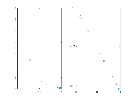
Suppose we have the X and Y values, and we can see or guess the functional form, but we don't know the constant values 10 and 5. We can estimate them from the data. We can do this using either the original data shown at the left, or the log(Y) transformed data shown at the right.
p1 = fitnlm(x,y,'y ~ b1*exp(b2*x)',[1 1])
p2 = polyfit(x,log(y),1); p2(2) = exp(p2(2))
p1 =
Nonlinear regression model:
    y ~ b1*exp(b2*x)

Estimated Coefficients:
          Estimate    SE    tStat    pValue
          ________    __    _____    ______
    b1       10       0      Inf       0
    b2       -5       0     -Inf       0

Number of observations: 10, Error degrees of freedom: 8
Root Mean Squared Error: 0
R-Squared: 1,  Adjusted R-Squared 1
F-statistic vs. zero model: Inf, p-value = 0
p2 =
   -5.0000   10.0000
Both fits give the same coefficients.
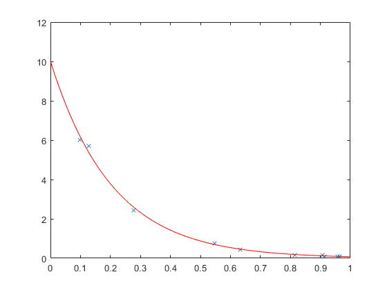
Some time ago, a MATLAB user reported that he was fitting this curve to his own data, and getting different parameter estimates from the ones given by other software. They weren't dramatically different, but larger than could be attributed to rounding error. They were different enough to raise suspicion. If we add a little noise to log(y), we can reproduce what the user saw.
y = exp(log(y) + randn(size(y))/10);
p1 = fitnlm(x,y,'y ~ b1*exp(b2*x)',[1 1])
p2 = polyfit(x,log(y),1); p2(2) = exp(p2(2))
xx = linspace(0,1)';
subplot(1,1,1)
plot(x,y,'x',  xx,predict(p1,xx),'r-')
p1 =
Nonlinear regression model:
    y ~ b1*exp(b2*x)

Estimated Coefficients:
          Estimate      SE        tStat       pValue
          ________    _______    _______    __________
    b1     10.015     0.34113      29.36    1.9624e-09
    b2    -4.8687     0.23021    -21.149     2.625e-08

Number of observations: 10, Error degrees of freedom: 8
Root Mean Squared Error: 0.141
R-Squared: 0.997,  Adjusted R-Squared 0.996
F-statistic vs. zero model: 1.91e+03, p-value = 1.91e-11
p2 =
   -4.8871   10.0008
Which estimates to believe? Well, it turns out that once you add noise, these models are no longer equivalent. Adding noise to the original data is one thing. Adding noise to the log data gives noise values that, back on the original scale, grow with the value of y. We can see the difference between the two more easily if we generate a larger set of data.
rng default
X = rand(100,1);
Y = 10*exp(-5*X);
subplot(1,2,1);
Y1 = Y + randn(size(Y))/5;
plot(X,Y1,'x', xx,10*exp(-5*xx),'r-');
subplot(1,2,2);
Y2 = exp(log(Y) + randn(size(Y))/10);
plot(X,Y2,'x', xx,10*exp(-5*xx),'r-');
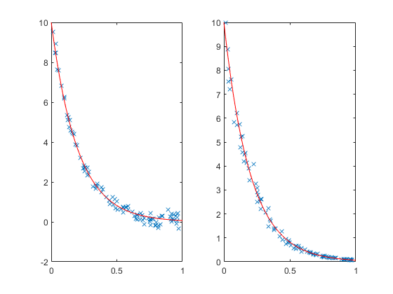
It's hard to see at the top of the plots, but near y=0 we can see that the noise is larger on the left than on the right. On the left the noise is additive. On the right, the noise is multiplicative.
Which model is correct or appropriate? We'd have to understand the data to decide that. One clue is that if negative values are plausible when the curve approaches zero, then an additive model may be appropriate. If the noise is more plausibly described in terms like +/- 10%, then the multiplicative model may be appropriate.
Now, not all models are easily transformed this way. A multiplicative model may still be appropriate even when no such simple transformation exists. Fortunately, the fitnlm function from the Statistics and Machine Learning Toolbox has a feature that lets you specify the so-called "error model" directly.
p1 = fitnlm(x,y,'y ~ b1*exp(b2*x)',[1 1],'ErrorModel','proportional')
p1 =
Nonlinear regression model:
    y ~ b1*exp(b2*x)

Estimated Coefficients:
          Estimate      SE       tStat       pValue
          ________    ______    _______    __________
    b1     9.9973     0.8188      12.21    1.8787e-06
    b2    -4.8771     0.1162    -41.973     1.144e-10

Number of observations: 10, Error degrees of freedom: 8
Root Mean Squared Error: 0.121
R-Squared: 0.974,  Adjusted R-Squared 0.97
F-statistic vs. zero model: 344, p-value = 1.75e-08
This model isn't exactly the same as the ones before. It's modeling additive noise, but with a scale factor that increases with the size of the fitted function. But rest assured, it takes into account the different noise magnitudes, so it may be useful for data having that characteristic.
Curve Fitting vs. Distribution Fitting
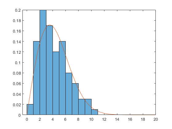
Now that I have your attention, though, I'd like to address another topic related to curve fitting. This time let's consider the Weibull curve.
rng default
x = wblrnd(5,2,100,1);
subplot(1,1,1)
histogram(x, 'BinEdges',0:14, 'Normalization','pdf')
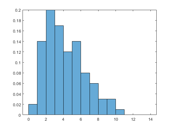
The Weibull density has this form:
X = linspace(0,20);
A = 5; B = 2;
Y = (B/A) * (X/A).^(B-1) .* exp(-(X/A).^B);
hold on
plot(X,Y)
hold off
Suppose we don't know the parameters A and B. Once again, there are two ways of estimating them. First, we could get the bin centers and bin heights, and use curve fitting to estimate the parameters.
heights = histcounts(x, 'BinEdges',0:14, 'Normalization','pdf');
centers = (0.5:1:13.5)';
fitnlm(centers,heights,@(params,x)wblpdf(x,params(1),params(2)),[2 2])
ans =
Nonlinear regression model:
    y ~ wblpdf(x,params1,params2)

Estimated Coefficients:
               Estimate      SE       tStat       pValue
               ________    _______    ______    __________
    params1     4.6535     0.18633    24.975    1.0287e-11
    params2     1.9091     0.10716    17.815    5.3598e-10

Number of observations: 14, Error degrees of freedom: 12
Root Mean Squared Error: 0.0182
R-Squared: 0.937,  Adjusted R-Squared 0.932
F-statistic vs. zero model: 197, p-value = 6.62e-10
The alternative is not to treat this like a curve fitting problem, but to treat it like a distribution fitting problem instead. After all, there is no need for us to artificially bin the data before fitting. Let's just fit the data as we have it.
fitdist(x,'weibull')
ans =
  WeibullDistribution

  Weibull distribution
    A = 4.76817   [4.29128, 5.29806]
    B = 1.96219   [1.68206, 2.28898]
It's much simpler to call the distribution fitting function than to set this up as a curve fitting function. But in case that doesn't convince you, I would like to introduce the concept of statistical efficiency. Notice that the distribution fitting parameters are closer in this case to the known values 5 and 2. Is that just a coincidence? A method is statistically more efficient than another if it can get the same accuracy using less data. Let's have a contest. We will fit both of these models 1000 times, collect the estimates of A, and see which one is more variable.
AA = zeros(1000,2);
for j=1:1000
    x = wblrnd(5,2,100,1);
    heights = histcounts(x, 'BinEdges',0:14, 'Normalization','pdf');
    f = fitnlm(centers,heights,@(params,x)wblpdf(x,params(1),params(2)),[2 2]);
    p = fitdist(x,'weibull');

    AA(j,1) = f.Coefficients.Estimate(1);
    AA(j,2) = p.A;
end
mean_AA = mean(AA)
std_AA = std(AA)
mean_AA =
    5.0145    4.9973
std_AA =
    0.3028    0.2566
We have a winner! Both values have a mean that is close to the known values of 5, but the values produced by distribution fitting are less variable.
Conclusion
When you approach a curve fitting problem, I recommend you consider a few things:
- Is this a curve fitting problem at all? If it involves the relationship between two variables, it's curve fitting. If it involves the distribution of a single variable, try to approach it as a distribution fitting problem.
- Is the function one that can transform to a simpler form, such as a linear relationship? If so, consider doing that to make the fitting process more efficient.
- However, consider the noise. Does the noise seem additive or multiplicative? Does the noise vary with the magnitude of Y? Are negative Y values plausible? These questions can help you decide whether to fit on the original or transformed scale, and whether to specify an error model.
What criteria do you use to choose a model for fitting your data? Let us know here.
- Category:
- Curve fitting,
- Statistics


Comments
To leave a comment, please click here to sign in to your MathWorks Account or create a new one.