 Cleve’s Corner: Cleve Moler on Mathematics and Computing
 The MATLAB Blog
 Guy on Simulink
 MATLAB Community
 Artificial Intelligence
 Developer Zone
 Stuart’s MATLAB Videos
 Behind the Headlines
 File Exchange Pick of the Week
 Hans on IoT
 Student Lounge
 MATLAB ユーザーコミュニティー
 Startups, Accelerators, & Entrepreneurs
 Autonomous Systems
 Quantitative Finance
 MATLAB Graphics and App Building
Displaying Fault Lines on a Geographic Globe using Mapping Toolbox
Guest blogger, Kelly Luetkemeyer, who is a senior software developer at MathWorks, returns with an article on displaying fault lines on a geographic globe. Kelly's previous articles included Tracking a Hurricane using Web Map Service, Visualizing the Gulf of Mexico Oil Slick using Web Map Service and Using RESTful Web Service Interface in R2014b MATLAB.
Contents
- Introduction
- Obtain Shapefile of Fault Lines from the United States Geological Survey
- Read Fault Lines Data from Shapefile
- Find Faults of Interest
- Display Fault Lines using Geographic Axes
- Display Fault Lines using Geographic Globe
- Find San Andreas Fault
- Add use of Custom Basemap from the USGS National Map
- Display San Andreas Fault on USGS Basemap using Geographic Axes
- Display San Andreas Fault on USGS Basemap using Geographic Globe
- Navigate to San Andreas Lake
- View San Andreas Fault in 3-D
- Add use of Custom Terrain from the USGS Earth Explorer
- Conclusion
Introduction
In R2020a, Mapping Toolbox introduced six new features for displaying data on a geographic globe.
- geoglobe - Create geographic globe
- geoplot3 - Geographic globe plot
- addCustomBasemap - Add use of custom basemap data on globe
- addCustomTerrain - Add use of custom terrain data on globe
- removeCustomBasemap - Remove use of custom basemap data on globe
- removeCustomTerrain - Remove use of custom terrain data on globe
This blog post illustrates how to plot fault lines on a 2-D geographic axes and a 3-D geographic globe. In geology, a fault is a fracture or discontinuity in a volume of rock and faults are one of the most important global geological hazards. Fault lines are plotted on a high zoom-level basemap hosted by Esri® and a custom basemap and custom terrain data from the United States Geological Survey (USGS).
Obtain Shapefile of Fault Lines from the United States Geological Survey
A shapefile of fault lines from the western United States can be obtained from https://earthquake.usgs.gov/static/lfs/nshm/qfaults/Qfaults_GIS.zip
Download and unzip the file. The shapefile is located in the folder: "GIS Files/Shapefile".
Read Fault Lines Data from Shapefile
Read the geographic data from the shapefile and convert to a geoshape vector for ease of use.
folder = "GIS Files/Shapefile";
shapefile = "QFaults.shp";
filename = fullfile(folder, shapefile);
faults = shaperead(filename,"UseGeoCoords",true);
faults = geoshape(faults);
Examine the number of elements and display the first element.
numberOfFaults = length(faults)
firstElenent = faults(1)
numberOfFaults =
112891
firstElenent =
1×1 geoshape vector with properties:
Collection properties:
Geometry: 'line'
Metadata: [1×1 struct]
Vertex properties:
Latitude: [41.8997 41.8914 41.8836 41.8800 NaN]
Longitude: [-120.2850 -120.2703 -120.2564 -120.2508 NaN]
Feature properties:
fault_name: 'Goose Lake graben faults (Goose Lake fault)'
sec_name: ''
fault_id: '828'
section_id: ''
Location: 'California'
linetype: 'Well Constrained'
age: 'late Quaternary'
dip: 'W'
slip_rate: 'Less than 0.2 mm/yr'
slip_sense: 'Normal'
scale: '1:250,000'
class: 'A'
mapped_cer: 'Good'
strike: ''
length: 0
cooperator: 'California Geological Survey'
earthquake: ''
fault_url: 'https://earthquake.usgs.gov/cfusion/qfault/show_report_AB_archive.cfm?fault_id=828§ion_id='
symbology: 'late Quaternary Well Constrained'
ref_id: '828'
Shape_Leng: 4.8044e+03
Find the number of unique locations.
numLocations = string(unique(faults.Location))'
numLocations =
  16×1 string array
    "Alaska"
    "Arizona"
    "California"
    "Colorado"
    "Hawaii"
    "Idaho"
    "Kansas"
    "Montana"
    "Nevada"
    "New Mexico"
    "Oklahoma"
    "Oregon"
    "Texas"
    "Utah"
    "Washington"
    "Wyoming"
Find Faults of Interest
Due to the size of the data, reduce the number of faults by finding faults that have a shape length greater than 10,000.
cutoffLength = 10000;
data = faults(faults.Shape_Leng > cutoffLength);
lat = data.Latitude;
lon = data.Longitude;
Display Fault Lines using Geographic Axes
Display the fault lines on a 2-D map. Construct a geographic axes using geoaxes and plot the data using geoplot. The geographic axes supports eleven different basemaps. The use of "darkmode" is popular in many applications. For visual contrast, select the "darkmode" (streets-dark) basemap. For a contrasting visual effect, display state boundaries in white. Read the state boundaries using shaperead.
states = shaperead("usastatelo.shp","UseGeo",true);
states = geoshape(states);
basemap = "streets-dark";
figure
gx = geoaxes("Basemap",basemap,"NextPlot","add");
geoplot(gx,lat,lon,"LineWidth",2)
geoplot(gx,states.Latitude,states.Longitude,"w")

Display Fault Lines using Geographic Globe
Display the fault lines on 3-D globe. 3-D visualizations with terrain provide more context for fault lines. The 2-D map is in a Web Mercator coordinate projection system which causes a scale distortion. Construct a geographic globe using geoglobe and plot the data using geoplot3. The fault lines contain many different segments, not one continuous line.
uif2 = uifigure;
g = geoglobe(uif2,"Basemap",basemap,"Terrain","none","NextPlot","add");
geoplot3(g,lat,lon,[],"LineWidth",2)
geoplot3(g,states.Latitude,states.Longitude,[],"w")

Find San Andreas Fault
The San Andreas fault is the most famous fault in the world and forms the tectonic boundary between the North American Plate and the Pacific Plate. The fault passes through California, a highly-populated state.
Search for the fault by using the fault_name property. Display the first element of the geoshape vector.
fault_name = "San Andreas";
index = contains(faults.fault_name,fault_name,"IgnoreCase",true);
san_andreas = faults(index);
lat = san_andreas.Latitude;
lon = san_andreas.Longitude;
firstElement = san_andreas(1)
firstElement =
1×1 geoshape vector with properties:
Collection properties:
Geometry: 'line'
Metadata: [1×1 struct]
Vertex properties:
Latitude: [1×39 double]
Longitude: [1×39 double]
Feature properties:
fault_name: 'San Andreas fault zone'
sec_name: 'Shelter Cove Section'
fault_id: '1'
section_id: 'a'
Location: 'California'
linetype: 'Moderately Constrained'
age: 'undifferentiated Quaternary'
dip: 'Vertical'
slip_rate: 'Greater than 5.0 mm/yr'
slip_sense: 'Right lateral'
scale: '1:100,000'
class: 'A'
mapped_cer: 'Good'
strike: 'N12°W'
length: 1082
cooperator: 'California Geological Survey'
earthquake: 'San Francisco earthquake'
fault_url: 'https://earthquake.usgs.gov/cfusion/qfault/show_report_AB_archive.cfm?fault_id=1§ion_id=a'
symbology: 'undifferentiated Quaternary Moderately Constrained'
ref_id: '1a'
Shape_Leng: 4.2662e+04
Add use of Custom Basemap from the USGS National Map
Geographic axes and geographic globe support custom basemaps. The USGS Shaded Topographic Map is a nice map for visualizing geophysical data. Use addCustomBasemap to add use of this map in geoaxes and geoglobe.
basemap = "usgstopo";
baseURL = "https://basemap.nationalmap.gov/ArcGIS/rest/services";
url = baseURL + "/USGSTopo/MapServer/tile/${z}/${y}/${x}";
attribution = "Credit: U.S. Geological Survey";
displayName = "USGS Shaded Topographic Map" ;
maxZoomLevel = 16;
addCustomBasemap(basemap,url,"Attribution",attribution, ...
    "DisplayName",displayName,"MaxZoomLevel",maxZoomLevel)
Display San Andreas Fault on USGS Basemap using Geographic Axes
Specify the USGS basemap by setting Basemap to the custom basemap name.
figure
gx = geoaxes("Basemap",basemap,"NextPlot","add");
geoplot(gx,lat,lon,"LineWidth",2,"Color","k")
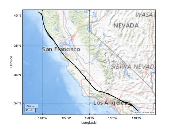
Display San Andreas Fault on USGS Basemap using Geographic Globe
Display the San Andreas fault line on a geographic globe. Specify the USGS basemap by setting Basemap to the custom basemap name. Specify no terrain and set the elevation of the fault line to one meter above the terrain.
uif1 = uifigure;
g = geoglobe(uif1,"Basemap",basemap,"Terrain","none","NextPlot","add");
h = 1;
geoplot3(g,lat,lon,h,"Color","k","LineWidth",2,"HeightReference","terrain");

Navigate to San Andreas Lake
According to wikipedia:
The fault was identified in 1895 by Professor Andrew Lawson of UC Berkeley,
who discovered the northern zone. It is often described as having been named
after San Andreas Lake, a small body of water that was formed in a valley
between the two plates. However, according to some of his reports from 1895
and 1908, Lawson actually named it after the surrounding San Andreas Valley.
The USGS basemap contains topographic information and placenames. The San Andreas Lake is near the San Francisco International Airport. Use the mouse to navigate to this region.

View San Andreas Fault in 3-D
The globe was constructed with the Terrain property set to "none". To view the San Andreas fault line in 3-D, set Terrain to "gmted2010" to use the Global Multi-resolution Terrain Elevation Data (GMTED2010). This dataset has a spatial resolution of 250 meters. Use the mouse to move and rotate the globe. Use the middle click plus drag or control plus left/right click plus drag to rotate the view.
g.Terrain = "gmted2010";
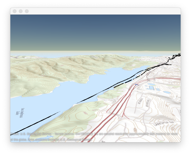
Add use of Custom Terrain from the USGS Earth Explorer
The globe supports use of custom terrain data in DTED format. DTED files can be obtained from the USGS Earth Explorer at https://earthexplorer.usgs.gov. Select your region using the map, select "Data Sets", "Digital Elevation", "SRTM", and then "SRTM Void Filled". The region selected covers San Francisco. The spatial resolution of DTED level-2 data is 30 meters, significantly better than the 250 meters resolution of GMTED2010. By using custom terrain, you can see greater detail and it minimizes obstruction of the view of the fault lines.
Use addCustomTerrain to add use of the custom terrain data. You only need to add use of custom terrain data once.
customTerrain = "sanfrancisco";
dtedfile = "n37_w123_1arc_v2.dt2";
addCustomTerrain(customTerrain,dtedfile)
View the region using the custom terrain. Notice the greater level of detail.
g.Terrain = customTerrain;

When finished, you can remove use of the custom basemap and custom terrain by using the functions removeCustomBasemap and removeCustomTerrain.
removeCustomBasemap(basemap)
removeCustomTerrain(customTerrain)
Conclusion
This post provides an introduction on how to plot fault lines on a 2-D geographic axes and on a 3-D geographic globe. How might you use these tools in your work? Do you have data to view in 3-D? What additional features would you like to see developed for the geographic globe?
Let us know here.
- Category:
- Mapping,
- New Feature


Comments
To leave a comment, please click here to sign in to your MathWorks Account or create a new one.