 Cleve’s Corner: Cleve Moler on Mathematics and Computing
 The MATLAB Blog
 Guy on Simulink
 MATLAB Community
 Artificial Intelligence
 Developer Zone
 Stuart’s MATLAB Videos
 Behind the Headlines
 File Exchange Pick of the Week
 Hans on IoT
 Student Lounge
 MATLAB ユーザーコミュニティー
 Startups, Accelerators, & Entrepreneurs
 Autonomous Systems
 Quantitative Finance
 MATLAB Graphics and App Building
Brad Efron’s Nontransitive Dice
Do not get involved in a bar bet with Brad Efron and his dice until you have read this.
Contents
Brad Efron
Bradley Efron is the Max H. Stein Professor of Humanities and Sciences, Professor of Statistics, and Professor of Biostatistics at Stanford. He is best known for his invention of the bootstrap resampling technique, which is a fundamental tool in computational statistics. In 2005, he received the National Medal of Science. But I think of him for something much less esoteric -- his nontransitive dice. And I also remember him as one of my roommates when we were both students at Caltech.
Brad's wager
If you come across Brad in a bar some night, he might offer you the following wager. He would show you four individual dice, like these.
![]()
Photo credit: http://www.grand-illusions.com
You would get to pick one of the dice. He would then pick one for himself. You would then roll the dice a number of times, with the player rolling the highest number each time winning a dollar. (Rolling the same number is a push. No money changes hands.) Do you want to play? I'll reveal the zinger -- no matter which of the four dice you choose, Brad can pick one that will win money from you in the long run.
Transitivity
A binary mathematical relationship, $\rho$, is said to be transitive if $x \ \rho \ y$ and $y \ \rho \ z$ implies $x \ \rho \ z$. Equality is the obvious example. If $x = y$ and $y = z$ then $x = z$. Other examples include greater than, divides, and subset.
On the other hand, a relationship is nontransitive if the implication does not necessarily hold. Despite their efforts to make it transitive, Facebook friend is still nontransitive.
Ordinarily, the term dominates, or beats is transitive. And, ordinarily, you might think this applies to dice games. But, no, such thinking could cost you money. Brad's dice are nontransitive.
Brad's dice
Here are the six values on the faces of Brad's four dice.
   A = [4 4 4 4 0 0];
   B = [3 3 3 3 3 3];
   C = [6 6 2 2 2 2];
   D = [5 5 5 1 1 1];
How do these compare when paired up against each other? It is obvious that A wins money from B because B rolls a 3 all of the time, while A rolls a winning 4 two-thirds of the time. The odds are 2:1 in A's favor. Similarly B's constant 3's dominate C's 2's two-thirds of the time. The odds are 2:1 in B's favor.
Comparing C with D is more complicated because neither rolls a constant value.. We have to compare each possible roll of one die with all the possible rolls of the other. That's 36 comparisons. The comparison is facilitated by constructing the following matrix. The comparison of a row vector with a column vector is allowed under MATLAB's new rules of singleton expansion.
Z = (C > D') - (C < D')
Z =
     1     1    -1    -1    -1    -1
     1     1    -1    -1    -1    -1
     1     1    -1    -1    -1    -1
     1     1     1     1     1     1
     1     1     1     1     1     1
     1     1     1     1     1     1
The result is a matrix Z with +1 where C beats D and a -1 where D beats C. There is a submatrix of -1s in the upper right, but no solid column or row. All that remains is to count the number of +1's and -1's to get the odds.
odds = [nnz(Z == +1) nnz(Z == -1)]
odds =
    24    12
There are twice as many +1s as -1s, so, again, the odds are 2:1 that C beats D.
But now how does D fair against A?
   Z = (D > A') - (D < A')
   odds = [nnz(Z == +1) nnz(Z == -1)]
Z =
     1     1     1    -1    -1    -1
     1     1     1    -1    -1    -1
     1     1     1    -1    -1    -1
     1     1     1    -1    -1    -1
     1     1     1     1     1     1
     1     1     1     1     1     1
odds =
    24    12
Again, there are twice as many +1s as -1s. The odds are 2:1 in D's favor.
To summarize, A beats B, B beats C, C beats D, and D beats A. No matter which die you choose, Brad can pick one that will beat it -- and by a substantial margin. It's like "Rock, Paper, Scissors" with a fourth option, but you have to make the first move.
Compare
Let's capture that comparison in a function. The function can print and label the matrix Z, as well as provide for pushes, which we'll need later.
type compare
function odds = compare(X,Y)
    Z = (X > Y') - (X < Y');
    odds = [nnz(Z==1) nnz(Z==0) nnz(Z==-1)];

    fprintf('\n         X  %3d %5d %5d %5d %5d %5d\n',X)
    fprintf('       Y\n')
    fprintf('   %5d  %5d %5d %5d %5d %5d %5d\n',[Y' Z]')
end
Use the function to compare A with C.
AvC = compare(A,C)
         X    4     4     4     4     0     0
       Y
       6     -1    -1    -1    -1    -1    -1
       6     -1    -1    -1    -1    -1    -1
       2      1     1     1     1    -1    -1
       2      1     1     1     1    -1    -1
       2      1     1     1     1    -1    -1
       2      1     1     1     1    -1    -1
AvC =
    16     0    20
Dividing out a common factor, that is odds of 4:5 against A.
The final possible comparison is B versus D. B's unimaginative play results in complete rows of +1 or -1.
BvD = compare(B,D)
         X    3     3     3     3     3     3
       Y
       5     -1    -1    -1    -1    -1    -1
       5     -1    -1    -1    -1    -1    -1
       5     -1    -1    -1    -1    -1    -1
       1      1     1     1     1     1     1
       1      1     1     1     1     1     1
       1      1     1     1     1     1     1
BvD =
    18     0    18
So B and D are an even match. Here is the complete summary of all possible pairings among Efron's Dice,
              A      B      C      D
        A           2:1    4:5    1:2
        B    1:2           2:1    1:1
        C    5:4    1:2           2:1
        D    2:1    1:1    1:2
Simulate
In case we don't believe these comparisons, or because we'd like to see the shape of the distribution, or just because it's fun, let's do some Monte Carlo simulations. Because 108 is divisible by 36, I'll make 108 rolls one game and simulate 10000 games. Here is the code.
type simulate
function simulate(X,Y)
    m = 108;   % Number of rolls in a single game.
    n = 10000; % Number of games in a simulation.
    s = zeros(1,n);
    for k = 1:n
        for l = 1:m
            i = randi(6);
            j = randi(6);
            if X(i) > Y(j)
                s(k) = s(k) + 1;
            elseif X(i) < Y(j)
                s(k) = s(k) - 1;
            % else X(i) == Y(j)
            % push counts as a roll
            end
        end
    end

    clf
    shg
    histogram(s)
    line([0 0],get(gca,'ylim'),'color','k','linewidth',2)
    title(sprintf('mean = %6.2f',mean(s)))
end
I'll initialize the random number generator so that I get the same results every time I publish this post.
rng(1)
Now verify that A beats B.
simulate(A,B);
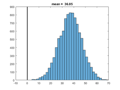
Sure enough, the 2:1 odds imply that A can be expected to be ahead by 108/3 dollars after 108 flips. There is a vertical black line at zero to emphasize that this isn't a fair game.
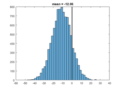
How about those 4:5 odds for A versus C? A can be expected to lose 108/9 dollars with 108 flips.
simulate(A,C)
Three dice nontransitive set
Efron's dice were introduced in a Scientific American article by Martin Gardner in 1970. Since then a number of people have found other sets of nontransitive dice with interesting properties. The Wikipedia article on nontransitive dice has an abundance of information, including the following set.
   A = [1 1 3 5 5 6];
   B = [2 3 3 4 4 5];
   C = [1 2 2 4 6 6];
This set is very close to a conventional set. The sum of the numbers on each die is 21, the same as a conventional die. And each die differs from a standard 1:6 die in only two places. Nevertheless, the set is nontransitive.
Since this is so close to a conventional set, we expect the odds to be closer to even. Let's see.
AvB = compare(A,B)
         X    1     1     3     5     5     6
       Y
       2     -1    -1     1     1     1     1
       3     -1    -1     0     1     1     1
       3     -1    -1     0     1     1     1
       4     -1    -1    -1     1     1     1
       4     -1    -1    -1     1     1     1
       5     -1    -1    -1     0     0     1
AvB =
    17     4    15
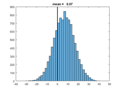
Since the dice have matching values, we have some zeros in the matrix. A has only 17 winning values compared to B's 15.
simulate(A,B)
Here is the result all three pairwise comparisons.
              A      B      C
        A          17:15  15:17
        B   15:17         17:15
        C   17:15  15:17


Comments
To leave a comment, please click here to sign in to your MathWorks Account or create a new one.