I have learned a lot more about Kuramoto oscillators since I wrote my blog post three weeks ago. I am working with Indika Rajapakse at the University of Michigan and Stephen Smale at the University of California, Berkeley. They are interested in the Kuramoto model because they are studying the beating of human heart cells. At this point we have some interesting results and some unanswered questions.

Contents

Kuramoto model

Recall that the Kuramoto model is a system of $n$ ordinary differential equations.

$$\dot{\theta_k} = \omega_k + \frac{\kappa}{n}\sum_{j=1}^n {\sin{(\theta_j-\theta_k)}}, \ k = 1,....,n.$$

Here $\theta_k(t)$ is a real-valued function of $t$ describing the phase of the $k$-th oscillator, $\omega_k$ is the intrinsic frequency of the $k$-th oscillator and the real scalar $\kappa$ is the strength of the coupling between the oscillators.

When $\kappa = 0$, the equations are linear and easily solved, and the oscillators are independent.

$$\theta_k(t)= \omega_k t$$

When $\kappa$ is increased beyond a critical point, the nonlinear term forces the phases of all the oscillators to approach a common limit.

Potential

Rajapakse and Smale have devised a new measure of synchronicity, the potential.

$$v = \frac{4}{n^2} \sum_k{ \sum_{j>k} \sin^2{ \left(\frac{\theta_j - \theta_k}{2} \right) }}$$

The $4/n^2$ normalizes the potential so that

$$0 \leq v \leq 1$$

The simulation is started with the $\theta_k$ equally spaced over the interval $[0,2\pi]$. This makes $v$ reach its maximum, $v = 1$, and indicates that the oscillators are completely out of sync. On the other hand, if we ever reach a point when all the $\theta_k$ are equal to a common value, then $v = 0$, indicating complete synchronization.

You can get to the Kuramoto ode system by taking $\partial v/\partial \theta_k$ and forming the gradient of the potential.

$$ \dot{\theta}-\omega = -\frac{\kappa n}{4}\nabla{v}$$

In my previous post, I described the "order parameter", shown in the simulator by the length of the cyan arrow. This varies between 0 initially and 1 at complete syncronization. One of the unanswered questions we have is exactly how the potential and the order parameter are related. A switch in kuramoto allows you to monitor either one.

Kuramoto simulator

The current version of my simulator is still called kuramoto, even though it replaces, and significantly improves, the version I described three weeks ago. The animation above shows it in action. There are five parameters controlled by sliders. The first three affect the dynamics of the system.

The vector omega is constant. Its components are randomly distributed uniformly in the interval [1-beta,1+beta] . This is the only source of randomness in the simulation. Setting beta to zero makes all the components of omega equal and eliminates any randomness.

The angular velocities of exp(i*theta) are color coded with the parula color map, blues for the fastest, yellows for the slowest, and greens in between.

Two more sliders affect the display, but not the dynamics of the system.

Since theta is real, exp(i*theta) lies on the unit circle. Display of a large number of oscillators moving around on the circle with different velocities is crowded. So, we display r*exp(i*theta) where r is normally distributed with mean one and standard deviation w. Setting w to zero forces the display to lie exactly on the circle.

Increasing step speeds up the simulation, but does not affect the computed solution, as long as it isn't too large. Setting step to zero pauses the simulation.

Snapshots

The following figures are static snapshots of the simulator output. All the snapshots are monitoring the potential. All are using the reference frame which rotates with the average theta, although this is hard to see in a static snapshot. The first four snapshots, with "many" oscillators, all have n = 100.

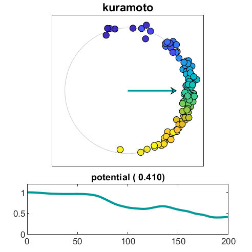
This first snapshot is the last frame of our animation. It has the default settings,

The oscillators are beginning to sychronize, although the potential has barely dropped below v = 0.5.

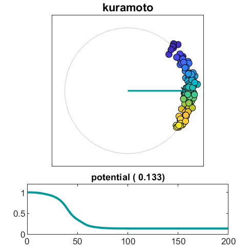
Increase coupling

Increase kappa from 0.15 to

The oscillators are cooperating, but the potential hovers above v = 0.13 .

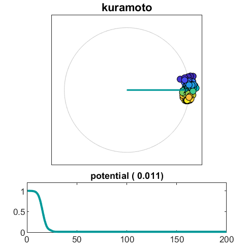
Increase coupling more and decrease variability

Set

This produces rapid syncronization and a potential near 0.01.

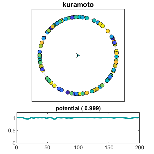
Confine display

Set

With beta at its maximum, there is lots of random action. The potential never drops below 0.99. But with the display width set to zero, all this turbulence is confined to the circle.

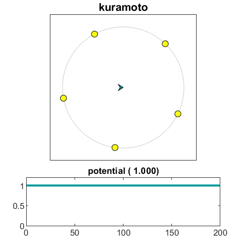
Few oscillators

Rajapakse and Smale are particularly interested in proving theorems about the behavior of the Kuramoto system when there are only a small handful of identical oscillators.

The five oscillators are represented initially as the vertices of a regular pentagon and, with both kappa and beta equal to zero, appear to stay there. It seems to be pretty boring.

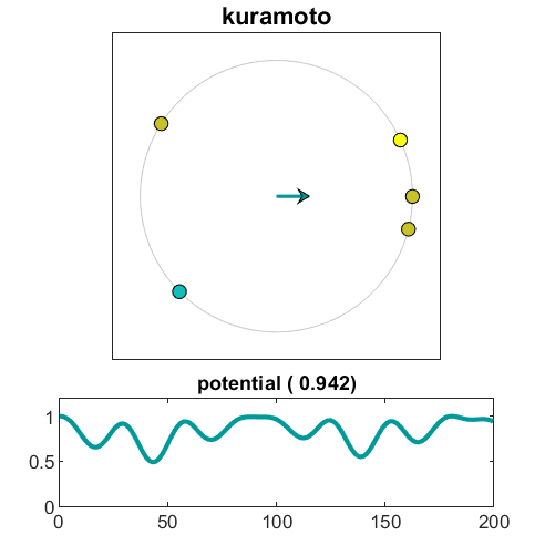
Add some variability

Try

Looks interesting. But, hold it, there is no coupling. As I said at the beginning, the exact solution is

$$\theta_k(t)= \omega_k t$$

with five different, but constant, omega(k). We are just seeing a five-term Fourier series. (I got fooled by this one.)

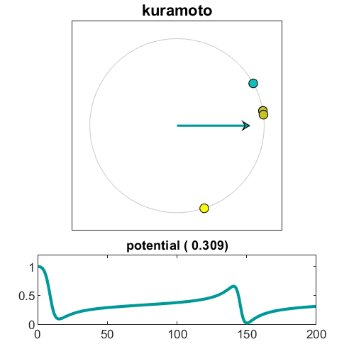
At last, some action

Try

There are actually five oscillators here. Three of them are on top of each other, but it's too soon to tell about the other two. Look at the potential.

Enough, already

I could go on like this all night, but enough for now. You can try some yourself by downloading the simulator from either its individual spot at MATLAB Central or as part of Cleve's Laborarory.

Preview

That snapshot I said is boring, isn't so boring after all. How do you arrange for a small handful of points to be equally spaced around the unit circle, and what are the consequences of any slight discrepancies. Remember pi $\ne \pi$.

References

Indika Rajapakse and Stephen Smale, "Emergence of function from coordinated cells in a tissue," Proceedings of the National Academy Sciences, 114 (7) 1462-1467, 2017, https://www.pnas.org/content/114/7/1462.short.

Dirk Brockman and Steven Strogatz, "Ride my Kuramotocycle", https://www.complexity-explorables.org/explorables/ride-my-kuramotocycle.

Steven Strogatz, Sync: The Emerging Science of Spontaneous Order, Hyperion, New York, 2003, link.

Steven Strogatz, On the Science of Sync. Video, http://www.cornell.edu/video/steven-strogatz-ted-talk-on-sync.

Steven Strogatz, "From Kuramoto to Crawford: Exploring the onset of synchronization in populations of coupled oscillators," Physica D 143, 1-20 (2000). link.

Yoshiki Kuramoto, Chemical Oscillations, Waves and Turbulence, Springer, 1984. https://www.springer.com/gp/book/9783642696916.

Get the MATLAB code

Published with MATLAB® R2018b