Interpolating Polynomials
John D'Errico is back today to talk about interpolating polynomials.
Contents
Introduction
I talked in my last blog about polynomial regression models. We saw some utility in polynomial models, and that increasing the order of the polynomial caused the errors to decrease. How far can we go? Can we reduce the errors to zero?
At some point, I might choose to increase the degree of the polynomial to one less than the number of data points. Assuming that my data have no replicated points, this is an interpolating polynomial that fits our data exactly, at least to within the double precision accuracy of our computations. A straight line can pass through any two points, a quadratic passes through three points, a cubic hits four points exactly, etc. If you prefer to think in terms of statistical degrees of freedom, if you have n points, a polynomial of order n-1 (with n coefficients) passes through your data exactly.
I've started this all out by talking about polynomial modeling in a least squares sense, or regression analysis. But really, I wanted to talk about interpolation, as opposed to the approximations provided by polynomial regression. Perhaps this was an indirect approach, but one of the things I feel important is to distinguish interpolation from the more general modeling/curve fitting tools used in mathematics. This difference is often unappreciated by many users of MATLAB.
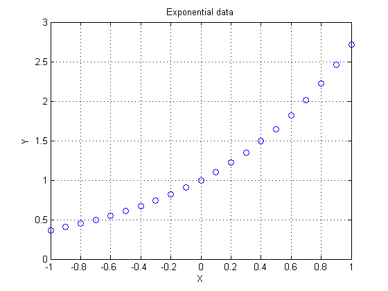
Let's start by sampling five points from an exponential function.
format short
x = (-2:1:2)';
y = exp(x);
plot(x,y,'o')
grid on

Exact Fit
While it is true that polyfit gives an exact fit with an order n-1 polynomial, a direct method is more efficient.
Build an interpolating polynomial using vander coupled with the use of backslash.
P = vander(x)\y
xev = linspace(-2,2,500)';
yev = polyval(P,xev);

plot(x,y,'ko',xev,yev,'r-')
grid on
title('Quartic polynomial through 5 points on exp(x)')
P =
    0.0492
    0.2127
    0.4939
    0.9625
    1.0000
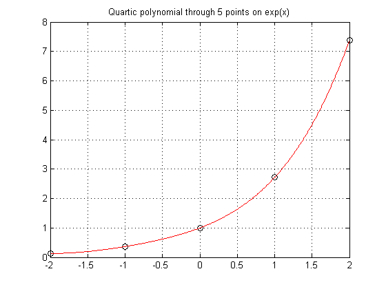
Many books teach you to use the Lagrange form for interpolation. I won't get into that here because I don't really advise the use of polynomials in general.
Interpolation should yield zero residuals at the data points
Verify that the residuals are essentially zero at the data points.
format long g
pred = polyval(P,x) - y
pred =
    -1.11022302462516e-016
    -1.11022302462516e-016
                         0
                         0
                         0
Does the Data Have Replicates?
Suppose I have two points with the same independent variable value, but distinct values for the dependent variable? Since for any given x, a single-valued function returns only a single value for the prediction, this must cause a problem. In this example, what value should I expect for an interpolant when x = 2? Should f(x) be 3 or 4?
x = [0 1 2 2 3 4]';
y = [1 2 3 4 5 6]';
plot(x,y,'-o')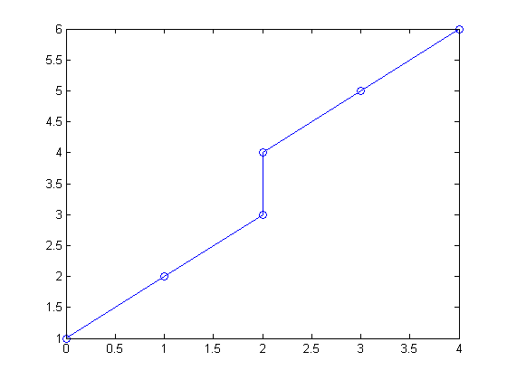
You can see a hint of the problem if you look at the rank of the Vandermonde matrix. The rank should have been 6, but the replicated point causes a singularity.
rank(vander(x))
ans =
     5
This singularity results in a rather useless polynomial.
P = vander(x)\y
Warning: Matrix is singular to working precision.
P =
   NaN
   NaN
   NaN
  -Inf
   Inf
     1
Average the Replicates
If the data truly is not single-valued, the common approach is to use a parametric relationship. (This is something to save for a possible future blog.)
Much of the time however, I just want to do something simple, like average the replicate points. consolidator, a tool I contributed to the File Exchange, can do just that. If you've never found or looked at the file exchange, please take some time to wander through the great tools there.
High Order Polynomials Not a Sure Bet
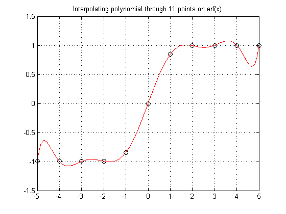
Sometimes polynomials don't do so well. It is important to know your data, know your problem. Here the data comes from a function known to be monotone increasing. Polynomials don't like to be monotone, so forcing a high order polynomial to interpolate such a function is a sure way to fail.
x = (-5:1:5)';
y = erf(x);

P = vander(x)\y
xev = linspace(-5,5,1000)';
yev = polyval(P,xev);

plot(x,y,'ko',xev,yev,'r-')
grid on
title('Interpolating polynomial through 11 points on erf(x)')
P =
     3.49245965480804e-020
      2.0991424886728e-005
    -1.58112816820803e-018
      -0.00119783140998794
     2.17562811018059e-017
        0.0239521737329468
    -9.91270557701033e-017
        -0.211403900317105
     1.85037170770859e-016
          1.03132935951897
                         0
Runge's Phenomenon
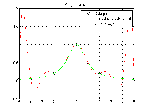
Runge found this example of a function that causes high order interpolating polynomials to fare very poorly.
x = (-5:1:5)';
y = 1./(1+x.^2);
P = vander(x)\y
xev = linspace(-5,5,1000)';
yev = polyval(P,xev);
ytrue = 1./(1+xev.^2);

plot(x,y,'ko',xev,yev,'r-.',xev,ytrue,'g-')
legend('Data points','Interpolating polynomial','y = 1./(1+x.^2)')
grid on
title('Runge example')
P =
    -2.26244343891403e-005
     1.04238735515992e-019
       0.00126696832579186
    -4.47734652027112e-018
       -0.0244117647058824
     5.61044648135202e-017
          0.19737556561086
    -2.38551402729053e-016
         -0.67420814479638
     1.38777878078145e-016
                         1
Numerical Problems
You also need to worry about numerical issues in high order polynomial interpolants. The matrices you would create are often numerically singular.
For example, the rank of the matrix vander(1:n) should be n. However, this fails when working in finite precision arithmetic.
rank(vander(1:10))
rank(vander(1:20))
rank(vander(1:30))
ans =
    10
ans =
     7
ans =
     6
Centering and scaling your data can improve the numerical performance of a high order polynomial to some extent, but that too has a limit. You are usually better off using other interpolation methods.
What can you do? You want to be able to interpolate your data. Polynomials seem like a good place to look, but they have their issues. High order polynomial interpolation often has problems, either resulting in non-monotonic interpolants or numerical problems. You might consider other families of functions to build your interpolant, for example trig or bessel functions, or orthogonal polynomials. Much depends on the relationship you want to model. KNOW YOUR PROBLEM!
By the way, for those who are interested in the methodology of modeling and curve fitting, I list a few ideas in this thread that should be of interest.
We can still do much with polynomials however. They form the basis for many modeling tools.
A nice trick is to go simple. Why use a single high order polynomial to interpolate our data? Instead, break the problem up and use smaller segments of low order polynomials, pieced together. In my next blog I'll begin talking about these piecewise interpolants. Until then please tell me here where you have found interpolating polynomials of use, or if you have found problems that they cannot solve.
- Category:
- Interpolation & Fitting




Comments
To leave a comment, please click here to sign in to your MathWorks Account or create a new one.