
Introduction to Market Basket Analysis
You probably heard about the "beer and diapers" story as the often quoted example of what data mining can achieve. It goes like this: some supermarket placed beer next to diapers and got more business because they mined their sales data and found that men often bought those two items together.
Today's guest blogger, Toshi Takeuchi, who works in the web marketing team here at MathWorks, gives you a quick introduction to how such analysis is actually done, and will follow up with how you can scale it for larger dataset with MapReduce (new feature in R2014b) in a future post.
Contents
Motivation: "Introduction to Data Mining" PDF
I have been interested in Market Basket Analysis not because I work at a supermarket but because it can be used for web usage pattern mining among many applications. Fortunately, I came across a good introduction in Chapter 6 (sample chapter available for free download) of Introduction to Data Mining. I obviously had to give it a try with MATLAB!
Let's start by loading the example dataset used in the textbook. Raw transaction data is turned into a binary matrix representation with 1 meaning the given item was in the given transaction, but otherwise 0.
transactions = {{'Bread','Milk'};...
    {'Bread','Diapers','Beer','Eggs'};...
    {'Milk','Diapers','Beer','Cola'};...
    {'Bread','Milk','Diapers','Beer'};...
    {'Bread','Milk','Diapers','Cola'}};

items = unique([transactions{:}]);
T = zeros(size(transactions,1), length(items));
for i = 1:size(transactions,1)
    T(i,ismember(items,transactions{i,:})) = 1;
end
disp(array2table(T,'VariableNames',items,'RowNames',{'T1','T2','T3','T4','T5'}))
          Beer    Bread    Cola    Diapers    Eggs    Milk
          ____    _____    ____    _______    ____    ____
    T1    0       1        0       0          0       1
    T2    1       1        0       1          1       0
    T3    1       0        1       1          0       1
    T4    1       1        0       1          0       1
    T5    0       1        1       1          0       1
Itemset and Support
Market Basket Analysis is also known as Association Analysis or Frequent Itemset Mining. Let’s go over some basic concepts: itemsets, support, confidence, and lift.
The column headers of the table shows all the items in this tiny dataset. A subset of those items in any combination is an itemset. An itemset can contain anywhere from zero items to all the items in the dataset.
0 items  --> null itemset (usually ignored)
1 item   --> 1-itemset
2 items  --> 2-itemset
      :
k items  --> k-itemset
This is, for example, a 3-itemset:
{Beer, Diapers, Milk}A transaction can contain multiple itemsets as its subsets. For example, an itemset {Bread, Diapers} is contained in T2, but not {Bread, Milk}.
Support count is the count of how often a given itemset appears across all the transactions. Frequency of its appearance is given by a metric called support.
Support = itemset support count / number of transactions
itemset = {'Beer','Diapers','Milk'}
% get col indices of items in itemset
cols = ismember(items,itemset);
N = size(T,1); fprintf('Number of transactions = %d\n',N)
% count rows that include all items
supportCount = sum(all(T(:,cols),2));
fprintf('Support count for this itemset = %d\n',supportCount)
itemSetSupport = supportCount/size(T,1);
fprintf('Support = %.2f\n',itemSetSupport)
itemset =
    'Beer'    'Diapers'    'Milk'
Number of transactions = 5
Support count for this itemset = 2
Support = 0.40
Association Rules, Confidence and Lift
Association rules are made up of antecedents (ante) and consequents (conseq) and take the following form:
{ante} => {conseq}A k-itemset where k > 1 can be randomly divided into ante and conseq to form such a rule. Here is an example:
ante = {'Diapers','Milk'}; % pick some subset itemset as |ante|
% get items not in |ante|
conseq = setdiff(itemset,ante);
fprintf('Itemset: {%s, %s, %s}\n', itemset{:})
fprintf('Ante   : {%s, %s}\n',ante{:})
fprintf('Conseq : {%s}\n',conseq{:})
fprintf('Rule   : {%s, %s} => {%s}\n', ante{:},conseq{:})
Itemset: {Beer, Diapers, Milk}
Ante   : {Diapers, Milk}
Conseq : {Beer}
Rule   : {Diapers, Milk} => {Beer}
You can think of this rule as "when diapers and milk appear in the same transaction, you see beer in the same transaction as well at some frequency". How do you determine which randomly generated association rules are actually meaningful?
The most basic measure of rules is confidence, which tells us how often a given rule applies within the transactions that contain the ante.
A given rule applies when all items from both antes and conseqs are present in a transaction, so it is the same thing as an itemset that contains the same items. We can use the support metric for the itemset to compute confidence of the rule.
Confidence = itemset support / ante support
cols = ismember(items,ante);
anteCount = sum(all(T(:,cols),2));
fprintf('Support Count for Ante = %d\n',anteCount)
anteSupport = anteCount/N;
fprintf('Support for Ante = %.2f\n',anteSupport)
confidence = itemSetSupport/anteSupport;
fprintf('Confidence = %.2f (= itemset support / ante support)\n',confidence)
Support Count for Ante = 3
Support for Ante = 0.60
Confidence = 0.67 (= itemset support / ante support)
Another measure of rules is lift. It compares the probability of ante and conseq happening together independently to the observed frequency of such a combination, as a measure of interestingness. If lift is 1, then the probabilities of ante and conseq occurring together is independent and there is no special relationship. If it is larger than 1, then lift tells us how strongly ante and conseq are dependent to each other. We can use respective support metrics to make this comparison.
Lift = itemset support / (ante support x conseq support)
cols = ismember(items,conseq);
conseqCount = sum(all(T(:,cols),2));
fprintf('Support Count for Conseq = %d\n',conseqCount)
conseqSupport = conseqCount/N;
fprintf('Support for Conseq = %.2f\n',conseqSupport)
lift = itemSetSupport/(anteSupport*conseqSupport);
fprintf('Lift = %.2f (= itemset support / (ante support x conseq support))\n',lift)
Support Count for Conseq = 3
Support for Conseq = 0.60
Lift = 1.11 (= itemset support / (ante support x conseq support))
Apriori Algorithm
Now that we know the basic concepts, we can define the goal of our analysis: finding association rules with a sufficient level of support (happens often enough) and confidence (association is strong). Lift can be a secondary measure to score the interestingness of the rules found.
- Generate frequent itemsets that clear the minimum support threshold recursively from 1-itemsets to higher level itemsets, pruning candidates along the way
- Generate rules that clear the minimum confidence threshold in a similar way
In a brute force method, you would calculate the support and confidence of all possible itemset combinations, but that would be computationally expensive, because the number of candidates grows exponentially.
The apriori algorithm addresses this issue by generating candidates selectively. To get an intuition, think about the frequency of an itemset that contains some infrequent items. That itemset will never be more frequent than the least frequent item it contains. So if you construct your candidates by combining the frequent itemsets only, starting from 1-itemset and continue to higher levels, then you avoid creating useless candidates.
Let's start with generating frequent itemsets and get their support measures. I wrote a couple of MATLAB functions to implement this algorithm.
minSup = 0.6; % minimum support threshold 0.6
[F,S] = findFreqItemsets(transactions,minSup);
fprintf('Minimum Support        : %.2f\n', minSup)
fprintf('Frequent Itemsets Found: %d\n', sum(arrayfun(@(x) length(x.freqSets), F)))
fprintf('Max Level Reached      : %d-itemsets\n', length(F))
fprintf('Number of Support Data : %d\n', length(S))
Minimum Support        : 0.60
Frequent Itemsets Found: 8
Max Level Reached      : 2-itemsets
Number of Support Data : 13
When we computed support for each itemset we evaluated, we stored the result in a Map object S. This is used for rule generation in order to avoid recalculating support as part of the confidence computation. You can now retrieve support for a given itemset with this object, by supplying the string representation of the itemset as the key. Let's try [2,4,6]:
itemset = [2,4,6];
fprintf('Support for the itemset {%s %s %s}: %.2f\n',items{itemset(:)},S(num2str(itemset)))
Support for the itemset {Bread Diapers Milk}: 0.40
This itemset clearly didn't meet the minimum support criteria of 0.60.
Rule Generation Algorithm
We saw earlier that you can generate rule candidates from frequent itemsets by splitting their contents into antes and conseqs, and computing their confidence.
If we generate every possible candidates by such brute force method, it will be very time consuming. Apriori algorithm is also used to generate rules selectively. Let's say that this rule has low confidence.
{Beer, Diapers} => {Milk}Then any other rules generated from this itemset that contain {Milk} in rule consequent will have low confidence.
{Beer} => {Diapers, Milk} {Diapers} => {Beer, Milk}Why? because support for those antes will be always greater than the initial ante {Beer, Diapers}, while the support for the itemset (hence also for the rule) remains the same, and confidence is based on the ratio of support between the rule and the ante.
We can take advantage of this intuition by first generating rules with only one item in conseq and drop those that don't meet the minimum criteria, and then merge those conseqs to generate rules with two items in conseq, and so forth.
Now we can generate association rules from the frequent itemsets we generated in the previous step.
minConf = 0.8; % minimum confidence threshold 0.8
rules = generateRules(F,S,minConf);
fprintf('Minimum Confidence     : %.2f\n', minConf)
fprintf('Rules Found            : %d\n\n', length(rules))

for i = 1:length(rules)
    disp([sprintf('{%s}',items{rules(i).Ante}),' => ',...
        sprintf('{%s}', items{rules(i).Conseq}),...
        sprintf('     Conf: %.2f ',rules(i).Conf),...
        sprintf('Lift: %.2f ',rules(i).Lift),...
        sprintf('Sup: %.2f',rules(i).Sup)])
end
Minimum Confidence     : 0.80
Rules Found            : 1

{Beer} => {Diapers}     Conf: 1.00 Lift: 1.25 Sup: 0.60
With a minimum support of 0.6 and a minimum confidence 0.8, we found only one rule that clears those thresholds: {Beer} => {Diapers}. The confidence is 1.00, which means we see diapers in all transactions that include beer, and the lift is 1.25, so this rule is fairly interesting.
Test Example: Congressional Voting Records
As a non-supermarket use case of Market Basket Analysis, the textbook uses the 1984 Congressional Voting Records dataset from the UCI Machine Learning Repository. We can test our code against the result in the textbook.
For the purpose of Market Basket Analysis, you can think of individual members of congress as transactions and bills they voted for and their party affiliation as items.
getData
       party        handicapped_infants    water_project_cost_sharing    adoption_of_the_budget_resolution
    ____________    ___________________    __________________________    _________________________________
    'republican'    'n'                    'y'                           'n'
    'republican'    'n'                    'y'                           'n'
    'democrat'      '?'                    'y'                           'y'
    'democrat'      'n'                    'y'                           'y'
    'democrat'      'y'                    'y'                           'y'
Now we generate frequent itemsets with a minimum support threshold of 0.3, but we need to use a slightly lower threshold because MATLAB uses double precision numbers.
minSup = 0.2988;
[F,S] = findFreqItemsets(votes,minSup);
fprintf('Minimum Support        : %.2f\n', minSup)
fprintf('Frequent Itemsets Found: %d\n', sum(arrayfun(@(x) length(x.freqSets), F)))
fprintf('Max Level Reached      : %d-itemsets\n', length(F))
fprintf('Number of Support Data : %d\n', length(S))
Minimum Support        : 0.30
Frequent Itemsets Found: 1026
Max Level Reached      : 7-itemsets
Number of Support Data : 2530
Then we generate some rules.
minConf = 0.9; % minimum confidence threshold 0.9
rules = generateRules(F,S,minConf);
fprintf('Minimum Confidence     : %.2f\n', minConf)
fprintf('Rules Found            : %d\n\n', length(rules))
Minimum Confidence     : 0.90
Rules Found            : 2942
Finally, let's compare our results with the results from the textbook.
testAntes = [7,21,27;5,11,23;6,15,16;22,31,32];
testConseqs = [2,1,2,1];
testConf = [0.91,0.975,0.935,1];

% Get the rules with 1-item conseq with party classification
dem = rules(arrayfun(@(x) isequal(x.Conseq,1),rules));
rep = rules(arrayfun(@(x) isequal(x.Conseq,2),rules));

% Compare the results
for i = 1:size(testAntes,1)
    rec = dem(arrayfun(@(x) isequal(x.Ante,testAntes(i,:)),dem));
    rec = [rec,rep(arrayfun(@(x) isequal(x.Ante,testAntes(i,:)),rep))];
    disp(['{', sprintf('%s, %s, %s',vars{rec.Ante}),'} => ',...
        sprintf('{%s}', vars{rec.Conseq})])
    fprintf('   Conf: %.2f Lift: %.2f Sup: %.2f\n',rec.Conf,rec.Lift,rec.Sup)
    if isequal(rec.Conseq,testConseqs(i));
        fprintf('   Correct!  Expected Conf %.2f\n\n',testConf(i))
    end
end
{El Salvador = Yes, Budget Resolution = No, Mx Missile = No} => {Republican}
   Conf: 0.91 Lift: 2.36 Sup: 0.30
   Correct!  Expected Conf 0.91

{Budget Resolution = Yes, Mx Missile = Yes, El Salvador = No} => {Democrat}
   Conf: 0.97 Lift: 1.59 Sup: 0.36
   Correct!  Expected Conf 0.97

{Physician Fee Freeze = Yes, Right To Sue = Yes, Crime = Yes} => {Republican}
   Conf: 0.94 Lift: 2.42 Sup: 0.30
   Correct!  Expected Conf 0.94

{Physician Fee Freeze = No, Right To Sue = No, Crime = No} => {Democrat}
   Conf: 1.00 Lift: 1.63 Sup: 0.31
   Correct!  Expected Conf 1.00
Visualization of Metrics
MATLAB has strong data visualization capabilities. Let's visualize conf, lift and support.
conf = arrayfun(@(x) x.Conf, rules); % get conf as a vector
lift = arrayfun(@(x) x.Lift, rules); % get lift as a vector
sup = arrayfun(@(x) x.Sup, rules); % get support as a vector
colormap cool
scatter(sup,conf,lift*30, lift, 'filled')
xlabel('Support'); ylabel('Confidence')
t = colorbar('peer',gca);
set(get(t,'ylabel'),'String', 'Lift');
title('1984 Congressional Voting Records')
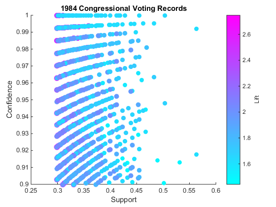
You see that rules we generated match with those in the textbook. The plot of support, confidence and lift is useful to identify rules that are high support, high confidence (upper right region of the plot) and high lift (more magenta). If you type gname into MATLAB prompt, you can interactively identify the indices of those points, and hit Enter to end the interactive session.
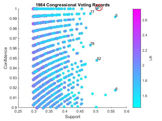
What was Rule 51? Let's find out.
disp('Rule ID = 51')
fprintf('{%s, %s} => {%s}, Conf: %.2f\n',...
    vars{rules(51).Ante(1)},vars{rules(51).Ante(2)},...
    vars{rules(51).Conseq},rules(51).Conf)
Rule ID = 51
{Budget Resolution = Yes, Physician Fee Freeze = No} => {Democrat}, Conf: 1.00
Closing
We used a small sample dataset in order to learn the basics of Market Basket Analysis. However, for real applications such as web usage pattern mining, we will typically be dealing with quite a large dataset. In a later post, I would like to figure out how to extend what we learned here with the help of MapReduce, introduced in R2014b. Any thoughts about your creative use of "Market Basket Analysis" with your data? Let us know here.
Appendix: Code used for this post
Here is the code used for this post.
findFreqItemsets() generates frequent itemsets using the Apriori method.
type findFreqItemsets.m
function [F,S,items] = findFreqItemsets(transactions,minSup,oneItemsets)
%FINDFREQITEMSETS generates frequent itemsets using Apriori method
%   |transactions| is a nested cell array of transaction data or a table
%   with |Value| column that contains such cell array. Each row contains a
%   nested cell array of items in a single transaction. If supplied as a
%   table, it also needs |Key| column with a cell array of transaction ids.
%
%   |minSup| is a scalar that represents the minimum support threshold.
%   Itemsets that meet this criteria are 'frequent' itemsets.
%
%   |oneItemSets| is an optional table that list all single items that
%   appear in |transactions| along with their frequencies. Items are listed
%   in |Key| column and corresponding counts in |Value| column.
%
%   |items| is a cell array of unique items.
%
%   |F| is a structure array of frequent itemsets that meet that
%   criteria. Items are represented as indices of cell arrat |items|.
%
%   |S| is a Map object that maps itemsets to their support values. Items
%   are represented as indices of cell arrat |items|.
%
%   To learn more about the underlying alogrithm itself, please consult
%   with Ch6 of http://www-users.cs.umn.edu/~kumar/dmbook/index.php

    % check the number of input arguments
    narginchk(2, 3)
    if iscell(transactions)
        transactions = table(num2cell(1:length(transactions))',transactions,'VariableNames',{'Key','Value'});
    end

    if nargin == 2
        items = transactions.Value;
        [uniqItems,~,idx] = unique([items{:}]');
        oneItemsets = table(uniqItems,num2cell(accumarray(idx,1)),'VariableNames',{'Key','Value'});
    end

    % get the total number of transactions
    N = height(transactions);
    % sort the tables
    transactions = sortrows(transactions,'Key');
    oneItemsets = sortrows(oneItemsets,'Key');
    % get all frequent 1-itemsets
    [F,S,items] = getFreqOneItemsets(oneItemsets,N,minSup);
    if isempty(F.freqSets)
        fprintf('No frequent itemset found at minSup = %.2f\n',minSup)
        return
    end

    % get all frequent k-itemsets where k >= 2
    k = 2;
    while true
        % generate candidate itemsets
        Ck = aprioriGen(F(k-1).freqSets, k);
        % prune candidates below minimum support threshold
        [Fk, support] = pruneCandidates(transactions,Ck,N,items,minSup);

        % update support data; if empty, exit the loop
        if ~isempty(support)
            % create a map object to store suppor data
            mapS = containers.Map();
            % convert vectors to chars for use as keys
            for i = 1:length(support)
                mapS(num2str(Ck(i,:))) = support(i);
            end
            % update S
            S = [S; mapS];
        else
            break;
        end
        % store the frequent itemsets above minSup
        % if empty, exit the loop
        if ~isempty(Fk)
            F(k).freqSets = Fk;
            k = k + 1;
        else
            break;
        end
    end


    function [F1,S,C1]= getFreqOneItemsets(T,N,minSup)
    % GETFREQ1ITEMSETS geneates all frequent 1-itemsets
    %   1-items are generated from 1-itemset table |T| and pruned with the
    %   minimum support threshold |minSup|.

        % get 1-itemset candidates
        C1 = T.Key;
        % get their count
        count = cell2mat(T.Value);
        % calculate support for all candidates
        sup = count ./N;
        % create a map object and store support data
        S = containers.Map();
        for j = 1:length(C1)
            S(num2str(j)) = sup(j);
        end
        % prune candidates by minSup
        freqSet = find(sup >= minSup);
        % store result in a structure array
        F1 = struct('freqSets',freqSet);
    end

    function [Fk,support] = pruneCandidates(T,Ck,N,items,minSup)
    %PRUNECANDIDATES returns frequent k-itemsets
    %   Compute support for each candidndate in |Ck| by scanning
    %   transactions table |T| to identify itemsets that clear |minSup|
    %   threshold

        % calculate support count for all candidates
        support = zeros(size(Ck,1),1);
        % for each transaction
        for l = 1:N
            % get the item idices
            t = find(ismember(items, T.Value{l}));
            % increment the support count
            support(all(ismember(Ck,t),2)) = support(all(ismember(Ck,t),2)) + 1;
        end
        % calculate support
        support = support./N;

        % return the candidates that meet the criteria
        Fk = Ck(support >= minSup,:);
    end

end
aprioriGen() is a helper function to findFreqItemsets() and generates candidate k-itemsets using the Apriori algorithm.
type aprioriGen.m
function Ck = aprioriGen(freqSets, k)
% APRIORIGEN generates candidate k-itemsets using Apriori algorithm
%   This function implements F_k-1 x F_k-1 method, which merges two pairs
%   (k-1)-itemsets to generate new k-itemsets if the first (k-2) items are
%   identical between the pair.
%
%   To learn more about the underlying alogrithm itself, please consult
%   with Ch6 of http://www-users.cs.umn.edu/~kumar/dmbook/index.php

    % generate candidate 2-itemsets
    if k == 2
        Ck = combnk(freqSets,2);
    else
        % generate candidate k-itemsets (k > 2)
        Ck = [];
        numSets = size(freqSets,1);
        % generate two pairs of frequent itemsets to merge
        for i = 1:numSets
            for j = i+1:numSets
                % compare the first to k-2 items
                pair1 = sort(freqSets(i,1:k-2));
                pair2 = sort(freqSets(j,1:k-2));
                % if they are the same, merge
                if isequal(pair1,pair2)
                    Ck = [Ck; union(freqSets(i,:),freqSets(j,:))];
                end
            end
        end
    end
end
generateRules() returns the association rules that meets the minium confidence criteria. It also uses aprioriGen() to generate rule candidates.
type generateRules.m
function rules = generateRules(F,S,minConf)
%GENERATERULES returns the association rules found from the frequent
%itemsets based on the minimum confidence threshold |minConf|.
%Association rules are expressed as {ante} => {conseq}.
%   |F| is a structure array of frequent itemsets
%   |S| is a Map object that maps itemsets to their support values
%   |rules| is a structure array of association rules that meet |minConf|
%   criteria, along with confidence, lift and support metrics.
%
%   To learn more about the underlying alogrithm itself, please consult
%   with Ch6 of http://www-users.cs.umn.edu/~kumar/dmbook/index.php

    rules = struct('Ante',{},'Conseq',{},'Conf',{},'Lift',{},'Sup',{});
    % iterate over itemset levels |k| where k >= 2
    for k = 2:length(F)
        % iterate over k-itemsets
        for n = 2:size(F(k).freqSets,1)
            % get one k-itemset
            freqSet = F(k).freqSets(n,:);
            % get 1-item consequents from the k-itemset
            H1 = freqSet';
            % if the itemset contains more than 3 items
            if k > 2
                % go to ap_genrules()
                rules = ap_genrules(freqSet,H1,S,rules,minConf);
            else
                % go to pruneRules()
                [~,rules] = pruneRules(freqSet,H1,S,rules,minConf);
            end
        end
    end

    function rules = ap_genrules(Fk,H,S,rules,minConf)
    %AP_GENRULES generate candidate rules from rule consequent
    %   |Fk| is a row vector representing a frequent itemset
    %   |H| is a matrix that contains a rule consequents per row
    %   |S| is a Map object that stores support values
    %   |rules| is a structure array that stores the rules
    %   |minConf| is the threshold to prune the rules

        m = size(H,2); % size of rule consequent
        % if frequent itemset is longer than consequent by more than 1
        if length(Fk) > m+1
            % prune 1-item consequents by |minConf|
            if m == 1
                [~,rules] = pruneRules(Fk,H,S,rules,minConf);
            end
            % use aprioriGen to generate longer consequents
            Hm1 = aprioriGen(H,m+1);
            % prune consequents by |minConf|
            [Hm1,rules] = pruneRules(Fk,Hm1,S,rules,minConf);
            % if we have consequents that meet the criteria, recurse until
            % we run out of such candidates
            if ~isempty(Hm1)
                rules = ap_genrules(Fk,Hm1,S,rules,minConf);
            end
        end
    end

    function [prunedH,rules] = pruneRules(Fk,H,S,rules,minConf)
    %PRUNERULES calculates confidence of given rules and drops rule
    %candiates that don't meet the |minConf| threshold
    %   |Fk| is a row vector representing a frequent itemset
    %   H| is a matrix that contains a rule consequents per row
    %   |S| is a Map object that stores support values
    %   |rules| is a structure array that stores the rules
    %   |minConf| is the threshold to prune the rules
    %   |prunedH| is a matrix of consequents that met |minConf|

        % initialize a return variable
        prunedH = [];
        % iterate over the rows of H
        for i = 1:size(H,1);
            % a row in H is a conseq
            conseq = H(i,:);
            % ante = Fk - conseq
            ante = setdiff(Fk, conseq);
            % retrieve support for Fk
            supFk =S(num2str(Fk));
            % retrieve support for ante
            supAnte =S(num2str(ante));
            % retrieve support for conseq
            supConseq =S(num2str(conseq));
            % calculate confidence
            conf = supFk / supAnte;
            % calculate lift
            lift = supFk/(supAnte*supConseq);

            % if the threshold is met
            if conf >= minConf
                % append the conseq to prunedH
                prunedH = [prunedH, conseq];
                % generate a rule
                rule = struct('Ante',ante,'Conseq',conseq,...
                    'Conf',conf,'Lift',lift,'Sup',supFk);
                % append the rule
                if isempty(rules)
                    rules = rule;
                else
                    rules = [rules, rule];
                end
            end
        end
    end

end
getData is a script that fetches the congressional voting data using the RESTful API access function webread() that was introduced in R2014b, and preprocesses the data for Market Basket Analysis.
type getData.m
% Let's load the dataset

clearvars; close all; clc

% the URL of the source data
url = 'https://archive.ics.uci.edu/ml/machine-learning-databases/voting-records/house-votes-84.data';

% define the function handle to process the data you read from the web
myreadtable = @(filename)readtable(filename,'FileType','text','Delimiter',',','ReadVariableNames',false);
% set up the function handle as |ContentReader| for |webread| function
options = weboptions('ContentReader',myreadtable);
% get the data
votes = webread(url,options);
% get the variable names
votes.Properties.VariableNames = {'party',...
    'handicapped_infants',...
    'water_project_cost_sharing',...
    'adoption_of_the_budget_resolution',...
    'physician_fee_freeze',...
    'el_salvador_aid',...
    'religious_groups_in_schools',...
    'anti_satellite_test_ban',...
    'aid_to_nicaraguan_contras',...
    'mx_missile',...
    'immigration',...
    'synfuels_corporation_cutback',...
    'education_spending',...
    'superfund_right_to_sue',...
    'crime',...
    'duty_free_exports',...
    'export_administration_act_south_africa'};

% display the small portion of the data
disp(votes(1:5,1:4))

% turn table into matrix
C = table2array(votes);
% create a logical array of yes votes
arr = strcmp(C(:,2:end), 'y');
% append logical array of no votes
arr = [arr, strcmp(C(:,2:end), 'n')];
% create a logical arrays of party affiliation
dem = strcmp(C(:,1),'democrat');
rep = strcmp(C(:,1),'republican');
% combine them all
arr = [dem,rep,arr];

% create cell to hold the votes of each member of congress
votes = cell(size(dem));
% for each member, find the indices of the votes
for i = 1:length(dem)
    votes{i} = find(arr(i,:));
end

% variable names that maps to the indices
vars = {'Democrat',...
    'Republican',...
    'Handicapped Infants = Yes',...
    'Water Project = Yes',...
    'Budget Resolution = Yes',...
    'Physician Fee Freeze = Yes',...
    'El Salvador = Yes',...
    'Religious Groups = Yes',...
    'Anti Satellite = Yes',...
    'Nicaraguan Contras = Yes',...
    'Mx Missile = Yes',...
    'Immigration = Yes',...
    'Synfuels Corp = Yes',...
    'Education Spending = Yes',...
    'Right To Sue = Yes',...
    'Crime = Yes',...
    'Duty Free = Yes',...
    'South Africa = Yes',...
    'Handicapped Infants = No'...,
    'Water Project = No',...
    'Budget Resolution = No',...
    'Physician Fee Freeze = No',...
    'El Salvador = No',...
    'Religious Groups = No',...
    'Anti Satellite = No',...
    'Nicaraguan Contras = No',...
    'Mx Missile = No',...
    'Immigration = No',...
    'Synfuels Corp = No',...
    'Education Spending = No',...
    'Right To Sue = No',...
    'Crime = No',...
    'Duty Free = No',...
    'South Africa = No'};
- Category:
- Big Data


Comments
To leave a comment, please click here to sign in to your MathWorks Account or create a new one.