
Automatic Differentiation in Optimization Toolbox™
This column is written by Alan Weiss, the writer for Optimization Toolbox documentation. Take it away, Alan.
Hi, folks. You may know that solving an optimization problem, meaning finding a point where a function is minimized, is easier when you have the gradient of the function. This is easy to understand: the gradient points uphill, so if you travel in the opposite direction, you generally reach a minimum. Optimization Toolbox algorithms are based on more sophisticated algorithms than this, yet these more sophisticated algorithms also benefit from a gradient.
How do you give a gradient to a solver along with the function? Until recently, you had to calculate the gradient as a separate output, with all the pain and possibility of error that entails. However, with R2020b, the problem-based approach uses automatic differentiation for the calculation of problem gradients for general nonlinear optimization problems. I will explain what all of those words mean. In a nutshell, as long as your function is composed of elementary functions such as polynomials, trigonometric functions, and exponentials, Optimization Toolbox calculates and uses the gradients of your functions automatically, with no effort on your part.
The "general nonlinear" phrase means that automatic differentiation applies to problems that fmincon and fminunc solve, which are general constrained or unconstrained minimization, as opposed to linear programming or least-squares or other problem types that call other specialized solvers.
Automatic differentiation, also called AD, is a type of symbolic derivative that transforms a function into code that calculates the function values and derivative values at particular points. This process is transparent; you do not have to write any special code to use AD. Actually, as you'll see later, you have to specify some name-value pairs in order not to have the solver use AD.
Contents
Problem-Based Optimization
The problem-based approach to optimization is to write your problem in terms of optimization variables and expressions. For example, to minimize the test function ${\rm fun}(x,y) = 100(y-x^2)^2 + (1-x)^2$ inside the unit disk $x^2+y^2\le 1$, you first create optimization variables.
x = optimvar('x');
y = optimvar('y');
You then create optimization expressions using these variables.
fun = 100*(y - x^2)^2 + (1 - x)^2;
unitdisk = x^2 + y^2 <= 1;
Create an optimization problem with these expressions in the appropriate problem fields.
prob = optimproblem("Objective",fun,"Constraints",unitdisk);
Solve the problem by calling solve, starting from x = 0, y = 0.
x0.x = 0;
x0.y = 0;
sol = solve(prob,x0)
Solving problem using fmincon.

Local minimum found that satisfies the constraints.

Optimization completed because the objective function is non-decreasing in
feasible directions, to within the value of the optimality tolerance,
and constraints are satisfied to within the value of the constraint tolerance.

sol =
  struct with fields:

    x: 0.7864
    y: 0.6177
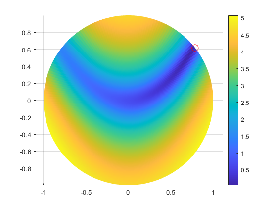
The solve function calls fmincon to solve the problem. In fact, solve uses AD to speed the solution process. Let's examine the solution process in more detail to see this in action. But first, plot the logarithm of one plus the objective function on the unit disk, and plot a red circle at the solution.
[R,TH] = ndgrid(linspace(0,1,100),linspace(0,2*pi,200));
[X,Y] = pol2cart(TH,R);
surf(X,Y,log(1+100*(Y - X.^2).^2 + (1 - X).^2),'EdgeColor','none')
colorbar
view(0,90)
axis equal
hold on
plot3(sol.x,sol.y,1,'ro','MarkerSize',10)
hold off
Effect of Automatic Differentiation
To examine the solution process in more detail, solve the problem again, this time requesting more solve outputs. Examine the number of iterations and function evaluations that the solver takes.
[sol,fval,exitflag,output] = solve(prob,x0);
fprintf('fmincon takes %g iterations and %g function evaluations.\n',...
    output.iterations,output.funcCount)
Solving problem using fmincon.

Local minimum found that satisfies the constraints.

Optimization completed because the objective function is non-decreasing in
feasible directions, to within the value of the optimality tolerance,
and constraints are satisfied to within the value of the constraint tolerance.

fmincon takes 24 iterations and 34 function evaluations.
The output structure shows that the solver takes 24 iterations and 34 function counts. Run the problem again, this time enforcing that the solver does not use AD.
[sol2,fval2,exitflag2,output2] = solve(prob,x0,...
    'ObjectiveDerivative',"finite-differences",'ConstraintDerivative',"finite-differences");
fprintf('fmincon takes %g iterations and %g function evaluations.\n',...
    output2.iterations,output2.funcCount)
plot([1 2],[output.funcCount output2.funcCount],'r-',...
    [1 2],[output.funcCount output2.funcCount],'ro')
ylabel('Function Count')
xlim([0.8 2.2])
ylim([0 90])
legend('Function Count (lower is better)','Location','northwest')
ax = gca;
ax.XTick = [1,2];
ax.XTickLabel = {'With AD','Without AD'};
Solving problem using fmincon.

Local minimum found that satisfies the constraints.

Optimization completed because the objective function is non-decreasing in
feasible directions, to within the value of the optimality tolerance,
and constraints are satisfied to within the value of the constraint tolerance.

fmincon takes 24 iterations and 84 function evaluations.

This time the solver takes 84 function counts, not 34. The reason for this difference is automatic differentiation.
The solutions are nearly the same with or without AD:
fprintf('The norm of solution differences is %g.\n',norm([sol.x,sol.y] - [sol2.x,sol2.y]))
The norm of solution differences is 1.80128e-09.
What Is Automatic Differentiation?
AD is similar to symbolic differentiation: each function is essentially differentiated symbolically, and the result is turned into code that MATLAB runs to compute derivatives. One way to see the resulting code is to use the prob2struct function. Let's try that on prob.
problem = prob2struct(prob);
problem.objective
ans =
  function_handle with value:
    @generatedObjective
prob2struct creates a function file named generatedObjective.m. This function includes an automatically-generated gradient. View the contents of the function file.
function [obj, grad] = generatedObjective(inputVariables)
%generatedObjective Compute objective function value and gradient
%
%   OBJ = generatedObjective(INPUTVARIABLES) computes the objective value
%   OBJ at the point INPUTVARIABLES.
%
%   [OBJ, GRAD] = generatedObjective(INPUTVARIABLES) additionally computes
%   the objective gradient value GRAD at the current point.
%
%   Auto-generated by prob2struct on 06-Oct-2020 09:01:35

%% Variable indices.
xidx = 1;
yidx = 2;

%% Map solver-based variables to problem-based.
x = inputVariables(xidx);
y = inputVariables(yidx);

%% Compute objective function.
arg1 = (y - x.^2);
arg2 = 100;
arg3 = arg1.^2;
arg4 = (1 - x);
obj = ((arg2 .* arg3) + arg4.^2);

%% Compute objective gradient.
if nargout > 1
    arg5 = 1;
    arg6 = zeros([2, 1]);
    arg6(xidx,:) = (-(arg5.*2.*(arg4(:)))) + ((-((arg5.*arg2(:)).*2.*(arg1(:)))).*2.*(x(:)));
    arg6(yidx,:) = ((arg5.*arg2(:)).*2.*(arg1(:)));
    grad = arg6(:);
end

end
While this code might not be clear to you, you can compare the AD gradient calculation to a symbolic expression to see that they are the same:
$\nabla({\rm fun}) = [-400(y-x^2)x - 2(1-x);\ 200(y-x^2)]$
The way that solve and prob2struct convert optimization expressions into code is essentially the same way that calculus students learn, taking each part of an expression and applying rules of differentiation. The details of the process of calculating the gradient are explained in Automatic Differentiation Background, which describes the "forward" and "backward" process used by most AD software. Currently, Optimization Toolbox uses only "backward" AD.
To use these rules of differentiation, the software has to have differentiation rules for each function in the objective or constraint functions. The list of supported operators includes polynomials, trigonometric and exponential functions and their inverses, along with multiplication and addition and their inverses. See Supported Operations on Optimization Variables and Expressions.
What Good is Automatic Differentiation?
AD lowers the number of function evaluations the solver takes. Without AD, nonlinear solvers estimate gradients by finite differences, such as $(f(x+\delta e_1) - f(x))/\delta ,$ where $e_1$ is the unit vector (1,0,...,0). The solver evaluates n finite differences of this form by default, where n is the number of problem variables. For problems with a large number of variables, this process requires a large number of function evaluations.
With AD and supported functions, solvers do not need to take finite difference steps, so the derivative estimation process takes fewer function evaluations and is more accurate.
This is not to say that AD always speeds a solver. For complicated expressions, evaluating the automatic derivatives can be even more time-consuming than evaluating finite differences. Generally, AD is faster than finite differences when the problem has a large number of variables and is sparse. AD is slower when the problem has few variables and has complicated functions.
What About Unsupported Operations?
So far I have talked about automatic differentiation for supported operations. What if you have a black-box function, one for which the underlying code might not even be in MATLAB? Or what if you simply have a function that is not supported for problem-based optimization, such as a Bessel function? In order to include such functions in the problem-based approach, you convert the function to an optimization expression using the fcn2optimexpr function. For example, to use the besselj function,
fun2 = fcn2optimexpr(@(x,y)besselj(1,x^2 + y^2),x,y);
fcn2optimexpr allows you to use unsupported operations in the problem-based approach. However, fcn2optimexpr does not support AD. So, when you use fcn2optimexpr, solving the resulting problem uses finite differences to estimate gradients of objective or nonlinear constraint functions. For more information, see Supply Derivatives in Problem-Based Workflow.
Currently, AD does not support higher-order derivatives. In other words, you cannot generate code for a second or third derivative automatically. You get first-order derivatives (gradients) only.
Final Thoughts
AD is useful for increased speed and reliability in solving optimization problems that are composed solely of supported functions. However, in some cases it does not increase speed, and currently AD is not available for nonlinear least-squares or equation-solving problems.
In my opinion, the most useful feature of AD is that it is utterly transparent to use in problem-based optimization. Beginning in R2020b, AD applies automatically, with no effort on your part. Let us know if you find it useful in solving your optimization problems by posting your comment here.
- Category:
- New Feature,
- Optimization


Comments
To leave a comment, please click here to sign in to your MathWorks Account or create a new one.