
Astrophotography with MATLAB: Imaging the Orion Nebula
Today I'd like to welcome two guest bloggers. David Garrison is a MATLAB Product Manager here at MathWorks. Andrei Ursache is a member of the Advanced Support Group with expertise in image acquisition and instrument control. This is the first in an occasional series of blog posts describing how they are doing astrophotography with MATLAB.
Thanks Loren. This is Dave. I'm going to tell you how we got started with this project and the equipment we're using. Andrei will then take over and tell you how we got our first deep-sky object images and how we've stacked and processed those images using MATLAB and the Image Processing Toolbox.
Contents
Our Interest in Astronomy
Readers of this blog may recall that in 2017, MathWorks was a sponsor of the Citizen CATE (Continental-America Telescopic Eclipse) Experiment -- a citizen science project run by the National Solar Observatory (NSO). The project's objective was to capture images of the sun's corona at sites along the eclipse path using a network of telescopes operated by volunteers. Those volunteers included high school and university groups, astronomy clubs, and individuals. MathWorks staff (including Andrei and me) manned three of the 67 sites observing the eclipse. The resulting 90 minutes of totality have helped solar astronomers better understand the dynamics of the sun's corona (MJ Penn et al. 2019 PASC).
There are a number of us here at MathWorks who are interested in amateur astronomy and astrophotography. None of us are astronomers by training but we all have telescopes at home that we use for observation and imaging of planets and deep-sky objects. It occurred to us that we could use MathWorks software to automate routine tasks and to do image stacking and post-processing. We put together a proposal to our management team to buy a MathWorks telescope that we could use to show how MATLAB and our other products could help amateur astronomers.
We bought our equipment in November, 2019 and spent the next few months learning about it. The images of the Orion Nebula were taken in January, 2020. Andrei will cover how we combined and processed those images in a minute but first some information about the equipment we selected.
The Equipment
To be successful in this project, we needed to find high quality equipment at a reasonable price -- something in the price range of a typical amateur astronomer. The three main pieces included the telescope optical tube assembly (OTA), the mount, and the camera. The OTA contains all the optical elements (mirrors and lenses). Eyepieces can be attached to the OTA for visual astronomy. Similarly, a camera can be attached to the telescope for astrophotography. The mount has motors that allow it to be moved in two directions - altitude (up/down) and azimuth (left/right). An important consideration for a mount is fine motor control. Cameras commonly used for astrophotography come in two types – digital single lens reflex (DSLR) cameras and dedicated astronomy cameras. Important considerations when choosing a camera for astrophotography include sensor format and size, sensitivity, dynamic range, and response linearity.
The assembled telescope that we bought is shown in the picture below. A DSLR camera is attached with a prime focus adapter.
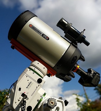
The Optical Tube Assembly (OTA). The requirements for the OTA were that it have a relatively large aperture for light collection and be light enough to be portable and easy to handle. We wanted high performance optics with high astrographic quality. We settled on an 8" Edge HD OTA from Celestron. The Edge HD is a Schmidt-Cassegrain design with aplanatic, flat-field optics. That means even stars at the edge of the field appear sharp and aberration-free. Out of the box it has a focal ratio of f/10 but can go down to f/7 with a focal reducer or as low as f/2 with an optional secondary mirror and third-party accessories. For astrophotography, lower focal ratios are better. We chose the Edge HD because it provided both high quality optics and the versatility to go to lower focal ratios in the future. To keep the OTA free from condensation and frost during cold or humid nights we also used a heated dew shield.
The Mount and Tripod. We wanted to purchase a high-quality mount with fine motor control. The mount we selected was the Skywatcher AZ-EQ6 PRO. In addition to having the specifications required for high-precision tracking, it has the added benefit that it can be configured in both equatorial mode (for astrophotography) or in Alt-Az mode (for visual astronomy). In the Alt-Az configuration, the mount can accommodate two saddles so you can mount two OTAs in parallel.
The Camera(s). To start, we decided to use two cameras that we already had in-house. The first is a Canon EOS 70D DSLR with a 22.5 x 15.0 mm APS-C format RGB sensor. It has a resolution of 5472 x 3648 pixels with an exposure range of 0.125 microseconds to 30 seconds or longer when triggered externally. The second is a FLIR Grasshopper3 5.0 MP Mono USB3 Vision camera with which we can acquire images at high frame rates directly in MATLAB using Image Acquisition Toolbox. This was the camera used for the Citizen CATE project. It has a Sony IMX250 CMOS monochrome sensor with a resolution of 2448 by 2028 pixels and a maximum frame rate of about 75 frames per second and an exposure range of 0.006 microseconds to 32 seconds. We have also purchased a computer-controlled filter wheel that will allow us to use the FLIR USB3 camera to image an object with red, green, and blue filters. Those color-filtered images can then be combined to get a color image. That will be one of our next steps.
Imaging the Orion Nebula
Thanks Dave. This is Andrei. For our first deep-sky object test run, we chose the Orion Nebula (Messier object M42), which is one of the brightest and easiest to image nebulae, visible in the northern hemisphere in the winter night sky.
Next I'm going to walk you through how we took images with a DSLR camera and telescope, and how we processed these images in MATLAB to create a composite image of the Orion Nebula.
Camera Configuration. We used a Canon D70 DSLR camera in a prime focus setup (using a telescope camera T-adapter and T-ring), with the image produced by the telescope being focused directly on the camera CMOS sensor. The images shown here were acquired with the telescope mount configured in equatorial mode and tracking in the right ascension axis at the sidereal rate.
A few tips when using a DSLR for astrophotography:
- Accurate polar alignment is essential to minimize drift and image artifacts during long exposures.
- Configure camera "mirror lockup" setting to On to reduce mechanical vibrations and image artifacts when taking a shot.
- Control camera shutter and change camera settings remotely and avoid touching the camera to reduce camera movements. Remote control can be done from a laptop connected to the camera via USB, a remote trigger, or a mobile app via a WiFi connection.
- If acquiring a small number of images, you might want to configure the camera "long exposure noise reduction" setting to On, to have the camera automatically subtract dark frames. As the camera takes an additional dark frame image for each shot, this effectively doubles the time for acquiring an image, but makes for simpler image processing later.
Reading the image files
A DSLR camera can save images in raw and/or JPEG format. To keep things simple, for this first blog post, we are using the JPG image files saved on the camera memory card. We will discuss importing images in RAW format in a future blog post.
For this image processing example, we selected a few images that were acquired with the following camera parameters:
- 20 second exposure time
- 1600 ISO
- long exposure noise reduction - On
% Specify image file names
filenames = ["_MG_7735.JPG", "_MG_7737.JPG", "_MG_7739.JPG"];
When read in MATLAB, each RGB image frame is a 3-D matrix. The first two dimensions are for y and x pixel coordinates, and the third dimension is for R, G, and B components. Let's read each image frame, convert its RGB values to double precision, and store all frame data in a 4-D matrix, where the fourth dimension is the frame index.
frameInfo = imfinfo(filenames(1));
frames = zeros([frameInfo.Height frameInfo.Width numel(filenames)]);
for ii = 1:numel(filenames)
    frame = imread(filenames(ii));
    frames(:,:,:,ii) = im2double(frame);
end

whos frames
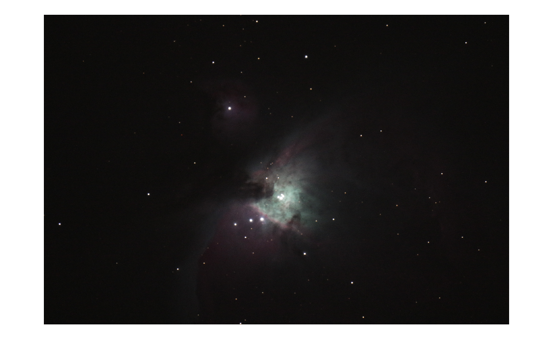
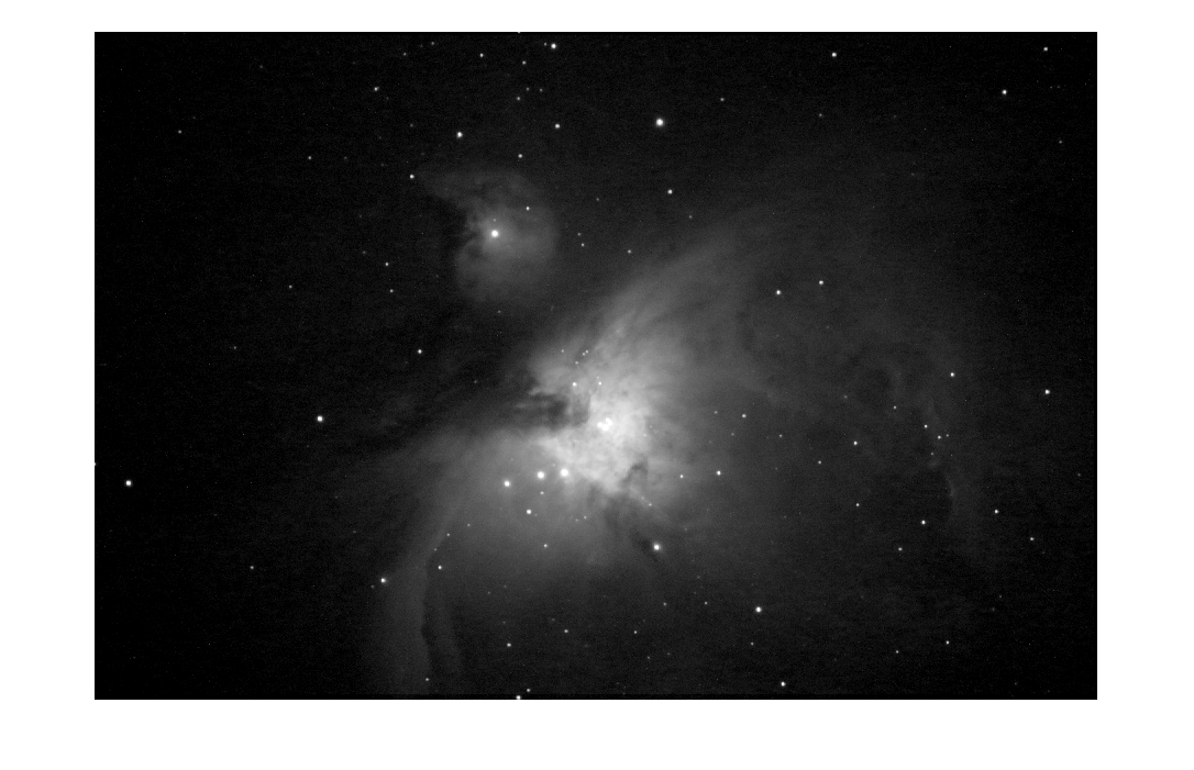
Here is the second frame:
imshow(frames(:,:,:,2))
In the unprocessed images, the core of the Orion Nebula is clearly visible, together with the Trapezium Cluster, named after the four primary stars at its center.
  Name           Size                       Bytes  Class     Attributes

  frames      3648x5472x3x3            1437253632  double
JPG image files saved by DSLR cameras can have the sRGB or Adobe RGB color space. Our camera was configured to save images with the Adobe RGB color space, which has gamma-adjusted R,G,B pixel values. For some technical image processing operations you want your data in linear RGB values. You can use the rgb2lin function for this purpose.
for ii = 1:numel(filenames)
    frames(:,:,:,ii) = rgb2lin(frames(:,:,:,ii),'ColorSpace','adobe-rgb-1998','OutputType','double');
end
Stacking the Images
To improve the image signal-to-noise ratio, one approach is to take multiple images and then create a composite image by combining them in software. A sequence of images taken with a telescope has small differences in alignment or position from image to image. In the case of an equatorial mount telescope, this can be caused by mount polar alignment error or by mount tracking errors. Seeing conditions can also cause local image distortions.
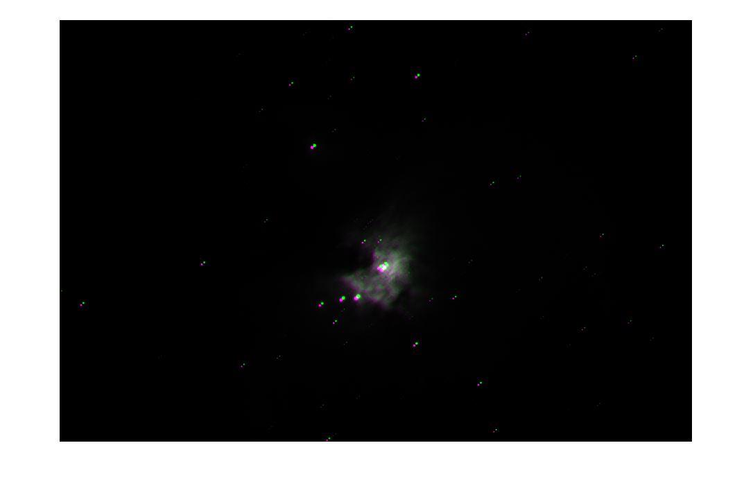
Here is a comparison of our first two frames using the imshowpair function. Visually, the difference between the two images appears to be a simple translation, as expected for tracking errors with an equatorial mount telescope.
imshowpair(frames(:,:,:,1),frames(:,:,:,2))
Before combining this set of images to create a composite image, we need to align or register them. The simplest way to get started with image registration is by using the Control Point Selection Tool, cpselect, which allows you to interactively register two images at a time. Using the second frame as a fixed reference, control points for each image pair were selected with cpselect, then exported and stored in the controlpoints.mat file. For more details refer to the Control Point Selection Procedure. In a future post, we will discuss other approaches to image registration.
% Load previously saved control points movingPoints1, fixedPoints1,
% movingPoints2, fixedPoints2
load controlpoints.mat

% cpselect(frames(:,:,:,1),frames(:,:,:,2))
tform = fitgeotrans(movingPoints1,fixedPoints1,'NonreflectiveSimilarity');
R = imref2d(size(frames(:,:,:,2)));
alignedFrames(:,:,:,1) = imwarp(frames(:,:,:,1),tform,'OutputView',R);

alignedFrames(:,:,:,2) = frames(:,:,:,2);

% cpselect(frames(:,:,:,3),frames(:,:,:,2))
tform = fitgeotrans(movingPoints2,fixedPoints2,'NonreflectiveSimilarity');
alignedFrames(:,:,:,3) = imwarp(frames(:,:,:,3),tform,'OutputView',R);
The simplest way to combine the registered images is to calculate the mean of all images over the frame index dimension.
img = mean(alignedFrames, 4);
Brighten detail in darker regions
To bring out detail in the fainter regions of the nebula, we need to brighten the image in those regions. One way to achieve this is to convert the RGB image to the HSL color space to obtain the hue, saturation, and lightness components, adjust the lightness, and then convert back to the RGB colorspace. To convert between RGB and HSL colorspaces we will use the convertToHSL and convertFromHSL helper functions, which are included at the end of this post.
[H,S,L] = convertToHSL(img);
Brighten lightness by taking the log of the pixel values in the lightness intensity image.
L2 = log(L);
Plot the histogram of the log-adjusted lightness. Because the original values were in the [0 1] range, the log of intensity has negative values (on the x-axis). The histogram y-axis is normalized as the ratio of the pixels with a certain intensity to the total number of pixels in the image. Most of the pixels correspond to the dark sky region.
histogram(L2,'Normalization','probability','EdgeColor','none');
xlabel('Adjusted lightness (a.u.)')
ylabel('Normalized pixel count')
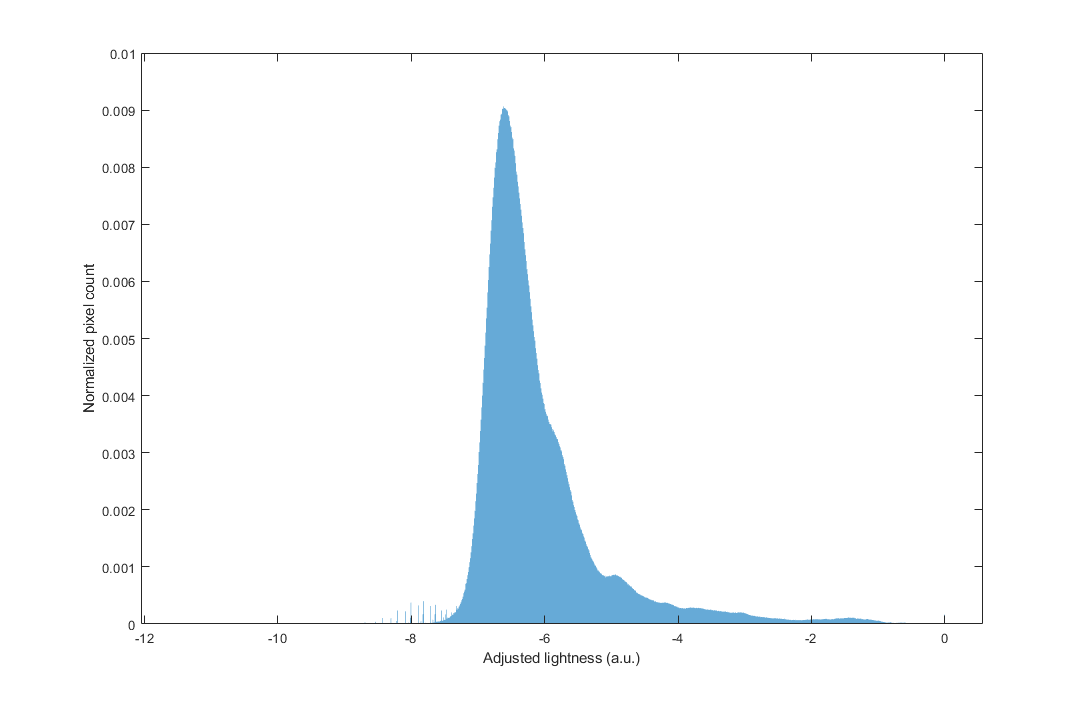
Adjust the black level of the lightness image to the intensity value in the dark sky region. Rescale the lightness values to the [0 1] interval and show the final adjusted lightness image.
blacklevel = -6.8;
L2 = rescale(L2,"InputMin",blacklevel);

imshow(L2,[0 1])
Details outside of the M42 Orion Nebula core are now visible. Neighboring nebula M43 and the dark dust lane between the two nebulas are also now apparent in the upper left quadrant of the image.
Create the final RGB image
To obtain the final RGB image we need to convert from the HSL colorspace, using the adjusted lightness, back to RGB. If desired, the color saturation of the final image can be adjusted by multiplying the saturation intensity image, SL, by a saturation factor. Multiplying by a value less than 1 reduces the color saturation.
saturation = 0.9;
S2 = saturation*S;
img2 = convertFromHSL(H,S2,L2);
To view the final image you can use the imshow function.
imshow(img2)
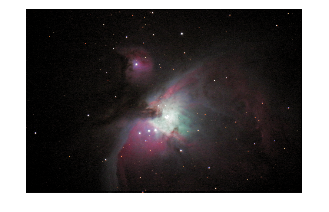
As compared to the original unprocessed RGB images, the brightened lightness also brings out the color in the darker regions of the nebula. Using a larger number of source images and using a range of exposure times can further improve the signal-to-noise ratio and the dynamic range.
Now we can save the final image as a JPEG file for sharing.
imwrite(img2,'orion_nebula.jpg')
What's Next?
In our next astrophotography session, we will pick a new deep-sky object and experiment further with combining images from the DSLR camera with a range of exposure times and ISO values. We also want to try out the FLIR USB3 camera and filter wheel and program an image acquisition sequence to control and acquire images directly from MATLAB.
In future posts, we will discuss how to automatically register and stack images, how to process images using dark and flat fields, how to acquire images from the camera directly in MATLAB, and other topics of interest in astrophotography. Once we get a little further into this project, we'll start posting tools we've created using MATLAB so that they are available to anyone who wants to use them.
Are You Interested in Astrophotography?
Have you done any imaging of the night sky? Have you used MATLAB to process astro images? Let us know about your experiences here.
Utility functions
The mentioned utility RGB/HSL color space conversion functions are included below:
function [H,SL,L] = convertToHSL(RGB)
%convertToHSL Converts image from RGB to HSL colorspace
% https://en.wikipedia.org/wiki/HSL_and_HSV

HSV = rgb2hsv(RGB);

% Convert from HSV to HSL
% HL = HV = H;
H = HSV(:,:,1);
SV = HSV(:,:,2);
V = HSV(:,:,3);

L = V-(0.5.*V.*SV);

SL = (V-L) ./ min(L, 1-L);
SL(L==0 | L==1) = 0;
end

function RGB = convertFromHSL(H,SL,L)
% convertFromHSL Converts image from HSL to RGB colorspace
% https://en.wikipedia.org/wiki/HSL_and_HSV

% Convert from HSL to HSV
% HV = HL = H;
V = L+SL.*min(L, 1-L);
SV = 2*(1-L./V);
SV(V==0) = 0;

HSV = cat(3,H,SV,V);

RGB = hsv2rgb(HSV);

end
- Category:
- Image Processing


Comments
To leave a comment, please click here to sign in to your MathWorks Account or create a new one.