
What is a leap second, anyway?
Today's post is brought to you from Peter Perkins, a member of the MathWorks development team.
Having worked on some of MATLAB's time and date functions, people at The MathWorks sometimes ask me questions about calendars and timekeeping. Often it goes something like this: in early January (or July), I stare at my phone for a moment during lunch and blurt out, "Bulletin C just published! No new leap second next June (or December)!", and then after awkward silence and "not again" looks from people who've heard this before, someone new says, "What the heck is a leap second, anyway?" I'm no expert, but my standard answer begins, "So, it turns out the earth is slowing down." The rest of the story follows.
Along the way, I'll show some uses of timetables and datetimes that are useful for working on time series data.
Table of Contents
So, it turns out that the earth is slowing down ... but not recently
For everyday purposes, we think of the length of a day as how long it takes for the sun to return to its zenith, in other words, for the earth to rotate once on its axis. We think of that as being 24 hours, but in fact it varies (as a consequence of Kepler's Second Law) with the seasons by about +30s/-21s because of the eccentricity of the earth's orbit (Kepler's First Law). It would be very inconvenient for the length of a "day" to vary by so much over the course of a year, because if we think of each day as 24*60*60=86400 seconds long, then the length of a second would need to be different in June than in December, and measuring elapsed time precisely would be impossible. Those seasonal effects on the length of a solar day can be smoothed out over the year, leading to the "mean solar day", which does not vary in length over a year. The time system based on mean solar days is known as "Universal Time" (UT).
The problem with UT is that, in addition to the "geometric effects" caused by an eccentric orbit, the earth's rotational speed is not constant over time. In fact, there is a long-term slowing in the rotation due to tidal interaction with the moon, and days are estimated to have grown longer by several hours over the past 600 million years. There is also a shorter-term component, smaller but in the opposite direction, believed to be due to melting of continental ice sheets over recent millennia. Historically speaking, the slowing rotation has meant that the length of a solar day has increased on average by about 1.4-1.7 ms every century. There are also seasonal cycles, and unpredictable fluctuations due to geological events and other causes. Over any given period on the order of a few decades, the length of even a mean solar day may increase, decrease, or both.
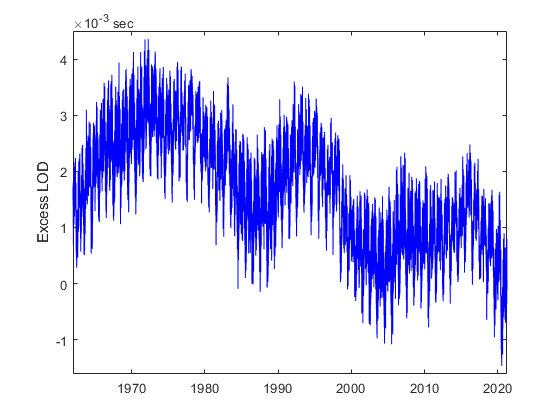
For scientific purposes, the second was defined in the 19th century as 1/86400th of a mean solar day, but if the length of a day fluctuates over time, what is a second actually equal to? That definition was based on astronomical data collected over the 18th and 19th centuries, effectively using a mean solar day from around 1820. But even by the late 19th century it was recognized that the then-current mean solar day was slightly longer than 86400s. By the 1940's and 1950's quartz and atomic clocks made the variations in the earth's rotational speed even more apparent, and led to more precise definitions of the length of one International System of Units (SI) second. Not suprisingly, the earth's rotation paid no attention to that, and the length of a mean solar day continued to fluctuate up and down over the 20th century. In recent decades, it has mostly been 1-3ms longer than 86400s. That difference is known as "excess Length Of Day (LOD)", and is published by the International Earth Rotation and Reference Systems Service.
file = "https://datacenter.iers.org/data/latestVersion/EOP_14_C04_IAU2000A_one_file_1962-now.txt";
IERSdata = readtable(file,"NumHeaderLines",14);
IERSdata.Properties.VariableNames([4 8]) = ["MJD" "ExcessLOD"];
IERSdata.Date = datetime(IERSdata.MJD,"ConvertFrom","mjd"); % modified Julian date -> datetime
IERSdata.ExcessLOD = seconds(IERSdata.ExcessLOD);
IERSdata = table2timetable(IERSdata(:,["Date" "ExcessLOD"]));
plot(IERSdata.Date,IERSdata.ExcessLOD,"b-");
ylabel("Excess LOD");
OK, sure, but what is a leap second, anyway?
A few extra ms seems unimportant, but the excess LOD accumulates. A clock that defines a "day" as 86400 SI seconds is effectively running fast with respect to the earth's rotation, gaining time with respect to the sun each day. For example, the time of day on that clock at which the sun appears at its zenith on June 21st would read a few tenths of a second later each successive year. Still, summing the excess LOD since the 1960's shows that the shift has been less than one minute, not even noticable for everyday purposes, so who cares?
IERSdata.CumulativeELOD = [0; cumsum(IERSdata.ExcessLOD(1:end-1))];
stackedplot(IERSdata,["ExcessLOD" "CumulativeELOD"]);

But over the course of centuries, the accumulated excess LOD could add up to the point where the sun at noon would noticeably no longer appear near its zenith. In other words, timekeeping based on 86400 SI seconds per day would drift away from physical experience, i.e. UT. This was regarded as a problem, despite the obvious fact that the variation in the sun's position at noon between cities at different "ends" of a time zone, or even between Standard Time and Daylight Saving Time in the same city, is much larger than the shift over the last century. Prior to 1972, various ad-hoc adjustments kept civil timekeeping more or less in sync with UT. By 1972, the current version of the system of time known as Coordinated Universal Time (UTC) was enacted, which uses 86400 SI seconds as defined by atomic clocks, but where an extra "leap second" adjustment is occasionally inserted to keep UTC approximately in sync with UT (UT1, more precisely). The idea is that because 86400s is a bit too short with respect to the earth's rotation, a UTC clock runs a bit too fast with respect to the sun overhead, so you just need to slow it down by making it tick off an extra second once in a while. It is also possible that the earth's rotation might speed up in the short term and make 86400s a bit too long, in which case a leap second might eventually need to be removed. So far, that has never happened; more about that below.
The earth's rotation is so unpredictable that the IERS announces leap seconds only six months in advance, in January and July. This particular timing makes it a scramble to get the latest information into each release of MATLAB. We try (check the second output of the leapseconds function).
Wait a second!
The current definition of UTC was adopted beginning at midnight on 1-Jan-1972, so I'll select only the post-1971 data.
IERSdata1972 = IERSdata(timerange("1-Jan-1972",Inf),"ExcessLOD");
The ad-hoc adjustments made to civil timekeeping during the 1960's meant that UTC differed from UT1 by about 45 milliseconds on 1-Jan-1972. But without leap second adjustments after 1972, accumulated excess LOD would have caused UTC to drift away from UT1 over the years. By 2017, the difference would have grown to about 26 sec.
DiffUT1_1972 = seconds(0.0454859);
IERSdata1972.UnadjDiff = DiffUT1_1972 + [0; cumsum(IERSdata1972.ExcessLOD(1:end-1))];
IERSdata1972(timerange("29-Dec-2016","4-Jan-2017"),:)
This growing difference is what leap seconds are designed to mitigate. The leapseconds function enumerates each of the "leap second events" that have occurred since 1972. The timetable returned by leapseconds contains the timestamp and a description of the event (so far, all leap seconds have been "positive" insertions, not "negative" removals), and also the cumulative number of leap seconds up to and including the event.
lsEvents = leapseconds()
Using the leap second timestamps to index into the timetable containing the LOD data, I'll add on what the unadjusted difference between UTC and UT1 would have been at each of those instants had leap seconds not been inserted.
lsEvents.UnadjDiff = IERSdata1972.UnadjDiff(lsEvents.Date)
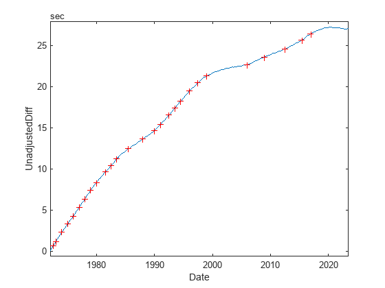
Looking at the unadjusted difference at each leap second event, it's apparent that leap seconds were inserted whenever the excess LOD would have accumulated by roughly one additional second. Plotting the leap seconds as points overlayed on the LOD data confirms that visually.
plot(IERSdata1972.Date,IERSdata1972.UnadjDiff);
ylabel("Cumulative Excess LOD");
hold on
plot(lsEvents.Date,IERSdata1972.UnadjDiff(lsEvents.Date),"r.");
hold off

Why leap seconds work
Each leap second is a instantaneous event that occurs at a specific time. Another way to represent them is as a variable appended to the LOD data that indicates the cumulative sum of leap seconds at any given date. Leap seconds occur at the end of a day, so first assign a value of 1 sec to the day after each event's date ...
IERSdata1972.Adjustment(lsEvents.Date+caldays(1)) = seconds(1);
IERSdata1972(timerange("29-Dec-2016","4-Jan-2017"),:)
... and then use a cumulative sum to fill in Adjustment at all other times in the data.
IERSdata1972.Adjustment = cumsum(IERSdata1972.Adjustment);
IERSdata1972(timerange("29-Dec-2016","4-Jan-2017"),:)
This new variable is defined at each time in the data, and so it can be used to compute the actual difference between UTC and UT1, given all the leap second adjustments, by subtracting it from the unadjusted difference computed above. By convention, it's computed as UT1-UTC, with the opposite sign as what we've been calling the unadjusted difference, and denoted as DUT1.
IERSdata1972.DUT1 = -(IERSdata1972.UnadjDiff - IERSdata1972.Adjustment);
IERSdata1972(timerange("29-Dec-2016","4-Jan-2017"),:)
The leap second adjustments are intended to keep UTC roughly in sync with UT1. Plotting Adjustment as a piecewise-constant step function over time illustrates how the adjustment works: the step function roughly approximates the accumulated excess LOD, so subtracting it keeps DUT1 small. Plotting DUT1 along the same time axis confirms that the adjustment keeps the difference less than 1 second.
stackedplot(IERSdata1972,{["UnadjDiff" "Adjustment"] "DUT1"});

Up time and down time
Leap seconds are inserted only when needed. Looking at some of the figures above, it appears that the average time between leap seconds has been increasing since 1972. Counting the number of events in each decade backs that up.
decade = discretize(lsEvents.Date,"decade","categorical");
histogram(decade);

To see why, we'll go back to the excess LOD data.
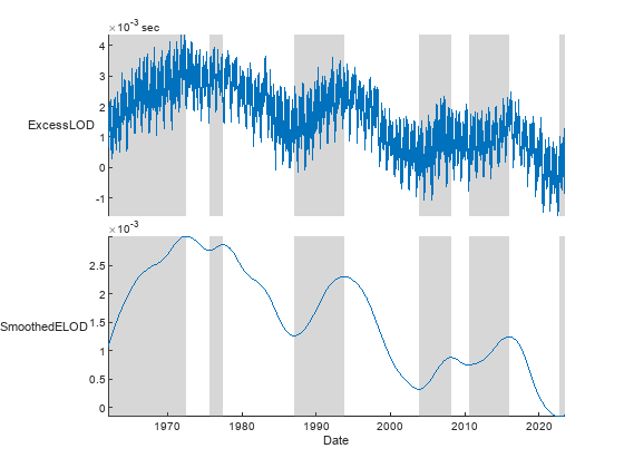
Since the 1960's, there have been several periods when excess LOD was decreasing over the short term. Smoothing the raw LOD data makes it easier to see the local behavior.
IERSdata.SmoothedELOD = smoothdata(seconds(IERSdata.ExcessLOD),"loess","SmoothingFactor",.4);
plot(IERSdata.Date,IERSdata.ExcessLOD,"b-");
hold on
plot(IERSdata.Date,IERSdata.SmoothedELOD,"g-","LineWidth",2);
hold off
ylabel("Excess LOD");

From the smoothed data, identify the peaks and troughs where the short-term trend changed direction, and get the date and the value of the smoothed excess LOD at each one.
peaks = find(islocalmax(IERSdata.SmoothedELOD));
troughs = find(islocalmin(IERSdata.SmoothedELOD));
Date = IERSdata.Date([peaks;troughs]);
Value = IERSdata.SmoothedELOD([peaks;troughs]);
Next I'll create a timetable containing the peak/trough events, and mark each of those peak/trough events on the plot. Each row of the timetable contains the event date, the type of event, and the excess LOD value at that event.
Type = categorical([zeros(size(peaks)); ones(size(troughs))],[0 1],["peak" "trough"]);
extremaEvents = sortrows(timetable(Date,Type,Value))
hold on
isPeak = (extremaEvents.Type =="peak");
plot(extremaEvents.Date(isPeak),extremaEvents.Value(isPeak),"y^","MarkerFaceColor","y");
plot(extremaEvents.Date(~isPeak),extremaEvents.Value(~isPeak),"yv","MarkerFaceColor","y");
hold off

The above is a plot of the excess LOD for individual days, and with a smoothed version that roughly tracks the yearly averages. What it says is, the day length averaged over the year has become approximately equal to, even slightly less than, 86400s over the last two years, meaning that the difference UTC-UT1 is actually flat or shrinking, not growing. The plot of cumulative excess LOD shown earlier indicates that it has already levelled out. That explains why no positive leap seconds have been added since Dec 2016. A shrinking UTC-UT1 raises the possibility that a negative leap second could eventually be needed. Not yet, hold your horses, but if this trend continues, it's conceivable that excess LOD could accumulate by something approaching -1s in a few years, and a negative leap second would then be necessary according to the definition of UTC. This has never happened before, and may cause a good deal of software a good deal of confusion (MATLAB will not be confused). A negative leap second just might be the motivation to finally abandon leap seconds. However, many experts believe that this trend will not continue, and is just part of a cycle.
There's a lot going on in that figure. There's excess LOD (essentially solar day length), its slope (how fast day length is changing), and its integral (the difference between UTC and UT1).
A race against time
From peak to trough, the excess LOD is decreasing, meaning that the earth's rotation is speeding up. I'll store the start and end of these decreasing periods in a table. The last peak has no matching trough; I'll use the last time in the data as the end time for the last interval.
StartDate = IERSdata.Date(peaks);
EndDate = [IERSdata.Date(troughs); IERSdata.Date(end)];
decreasingEvents = table(StartDate,EndDate)
hold on
startEnd = [decreasingEvents.StartDate decreasingEvents.EndDate];
h = fill(startEnd(:,[1 2 2 1]),[-.002 -.002 .005 .005],"red","FaceAlpha",.2,"LineStyle","none");
hold off

Finally, I'll compute the average decrease in excess LOD during each interval (in units of "seconds of daily excess LOD" per year), and add that information to the interval events in the table.
dTime = decreasingEvents.EndDate - decreasingEvents.StartDate;
dExcess = IERSdata.SmoothedELOD(decreasingEvents.EndDate) - IERSdata.SmoothedELOD(decreasingEvents.StartDate);
decreasingEvents.AnnualAvgDecrease = seconds(dExcess ./ years(dTime))
In other words, the mean solar day, averaged over an entire year, has been decreasing over the last few years by about 0.3ms per year. As we saw above, it is currently very close to 86400s. If the recent decrease continues, and a year from now the mean solar day is 0.3ms less than 86400s, that means that negative excess LOD would accumulate at around a tenth of a second a year. But at that rate it would take close to ten years before a negative leap second would be needed.
No time to lose
Will the earth stop speeding up? In the long term, yes. You can't win against tidal interaction.
In many recent years there have been very short periods when the raw excess LOD was significantly negative, relatively speaking. These are only brief fluctuations, but during those periods, the earth was rotating as much as 1.5ms faster than 86400 SI seconds.
plot(IERSdata.Date,IERSdata.ExcessLOD,"b-");
ylabel("Excess LOD");
hold on
line(IERSdata.Date([1 end]),[0 0],"Color","k","LineStyle",":")
hold off
ylabel("Excess LOD");

I'll identify the years in which the excess LOD was less than -0.5ms on any day, find the minimum excess LOD in each of those years, and create a table of those minimum values.
negLOD = IERSdata(IERSdata.ExcessLOD < milliseconds(-0.5),"ExcessLOD");
groupsummary(negLOD,"Date","year","min")
So what's going to happen next year? The whole reason why leap seconds are announced only six months in advance is because it's difficult to predict changes in the earth's rotational speed with any accuracy. But although the IERS doesn't predict excess LOD very far in the future, they do publish predictions of DUT1 going out one year.
t = readtable("https://datacenter.iers.org/data/latestVersion/finals.all.iau2000.txt");
t = t(:,[3 10 12]);
t.Properties.VariableNames = ["Date" "DUT1" "LOD"];
t.Date = datetime(t.Date,"ConvertFrom","mjd");
t.DUT1 = seconds(t.DUT1);
t.LOD = milliseconds(t.LOD);
t = t(t.Date >= "1-Jan-2020",:)
predictions = (t.Date >= "1-Apr-2021");
plot(t.Date(~predictions),t.DUT1(~predictions),'b', ...
t.Date(predictions), t.DUT1(predictions), 'r');
ylabel("DUT1")
legend(["Actual" "Predicted"],"Location","northwest")

Remember, DUT1 is UT1-UTC, and positive leap seconds are added when DUT1 becomes less than about -0.5s. The slope over the past year shows that solar day length has been greater than, then less than, and then roughly equal to 86400s. The slope over the next year predicts that solar day length will be less than, then equal to, and then greater than 86400s. If correct, that means ... no leap seconds, negative or positive, for some time! It will be interesting to keep an eye on this over the next few years. If the pattern since 1970 continues, negative leap seconds will be needed, but the question is when: will excess LOD turn up again soon as part of the recent decadal cycles, or continue to decrease as it has since 2015?
Reading time
A large part of what I know about time systems and leap seconds comes from these amazingly comprehensive pages by Steve Allen at UCO/Lick Observatory. Other very readable accounts of the history of UTC and leap seconds are by Levine, McCarthy, Quinn, and Nelson et al.
Time to wrap up
The main way that leap seconds rear their ugly head is when you calculate the difference between two instants in time that span one or more leap seconds. In MATLAB, you can opt in to using leap seconds in your datetime calculations by using UTCLeapSeconds to create your datetimes:
datetime(2016,12,31,36,0,0,"TimeZone","UTCLeapSeconds") - datetime(2016,12,31,12,0,0,"TimeZone","UTCLeapSeconds")
But we found that most people would just be annoyed to see an extra second creeping in apparently at random, so without explicitly asking for leap second accounting, you'd see
datetime(2016,12,31,36,0,0,"TimeZone","UTC") - datetime(2016,12,31,12,0,0,"TimeZone","UTC")
and the same for any other time zone such as America/New_York. (We also discovered that many people find an extra hour or a missing hour twice a year annoying, so you also have to opt in to Daylight Saving Time by using a time zone.)
Does your work require leap seconds in calculations and have you used UTCLeapSeconds? Or do you just find them annoying? Should leap seconds be abandoned? Unlike UTC, the GPS time system does not insert leap seconds, and so it is a "uniform" time system, but diverges from UTC by 1s each time a leap second is inserted in UTC. Does your work use GPS time? Let us know your MATLAB time experiences (woes?) here.
- Category:
- Data types,
- Time


Comments
To leave a comment, please click here to sign in to your MathWorks Account or create a new one.