Mathematical Recreations: Tweetable Game Of Life

Today I’d like to introduce a guest blogger, Matt, who is consultant over in The MathWorks UK. Some of you may have come across his customer projects and series of demos on using MATLAB in Physics. He’s going to talk about an interesting one line MATLAB program.

Contents

Introduction

One Saturday afternoon I saw a link on Hacker News to a YouTube video showing Conway's Game of Life in one line of APL. This made me wonder whether MATLAB® could perform as well.

The answer: maybe not quite a single line, but definitely a tweet.

The code is reproduced below:

s=[1 1 1]';
n=@(a)conv2(s,s',1*a,'same')-a;
lf=@(a)n(a)==2&a|n(a)==3;
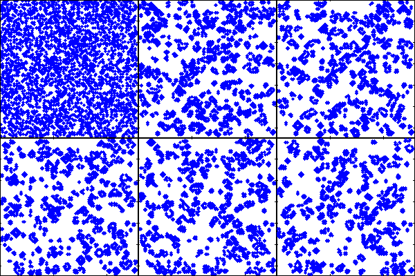
a=rand(128)>0.8;
for ii=1:500,spy(a);drawnow;a=lf(a);end

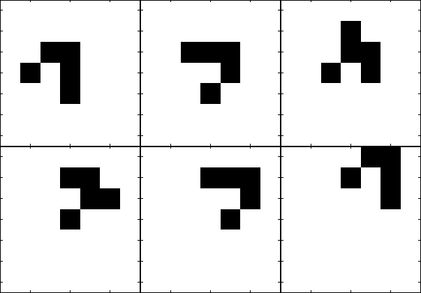
In the code below I've commented out the population initialisation and visualisation code and replaced it with various alternatives for this published version, together with an animated gif of the output.

A = accumarray([3 3; 3 4; 4 2; 4 4; 5 4],1,[7 7]);
imagesc(~A); colormap(gray);
for ii=1:9,imagesc(~A);drawnow;A=lf(A);end

In this post I'll show the evolution of the code from initial conception to finished version, and how thinking in matrices can lead to new algorithms.

Conway's Game Of Life

Conway's Game of Life is a two-dimensional cellular automation that demonstrates complex behaviour.

It consists of a grid of cells, each of which may be in one of two possible states, 0 ('dead') or 1 ('alive'). The state of each cell in the next iteration of the game is dependent on the state of the surrounding eight cells as follows:

The core of the algorithm consists of two steps:

Calculating The Number Of Neighbours

To calculate the number of neighbours for each cell one approach would be to loop over each cell in the array, add up the number of live cells in the surrounding 3x3 square, and finally subtract the state of the cell itself.

The YouTube video used the different approach of creating 8 copies of the original array, offseting each by a step horizontally and/or vertically and then summing the arrays.

The key part of development of my algorithm was to realise that this looping-with-sum-over-neighbourhood is just a 2D convolution. In MATLAB we can do a 2D convolution using conv2.

S = [1 1 1; 1 0 1; 1 1 1]
neighbours=@(a) conv2(double(a),S,'same')

S =
     1     1     1
     1     0     1
     1     1     1
neighbours = 
    @(a)conv2(double(a),S,'same')

The 'same' argument is to restrict the output of conv2 to be the same size as the original input matrix.

For example:

b = rand(5)>0.5
neighbours(b)

b =
     0     0     1     1     1
     1     1     0     1     0
     1     0     1     0     1
     0     1     1     0     0
     0     0     1     0     1
ans =
     2     3     3     3     2
     2     4     5     5     4
     3     6     4     4     1
     2     4     3     5     2
     1     3     2     3     0

Calculating The Next State

After calculating the number of neighbours, the next step is to use it to determine the next state using the rules of Conway's Game of Life.

life = @(a) (neighbours(a)==2 & a)...  % Rule for 2 neighbours
    | (neighbours(a)==3)               % Rule for 3 neighbours
b
life(b)

life = 
    @(a)(neighbours(a)==2&a)|(neighbours(a)==3)
b =
     0     0     1     1     1
     1     1     0     1     0
     1     0     1     0     1
     0     1     1     0     0
     0     0     1     0     1
ans =
     0     1     1     1     1
     1     0     0     0     0
     1     0     0     0     0
     0     0     1     0     0
     0     1     1     1     0

Let's use this as a reference implementation to test that modifications to the function do the same thing:

t = @(fOrig,f,a) assert(all(all(fOrig(a) == f(a))));

Reducing The Size

Twitter allows users to post 'tweets' of up to 140 characters in length. Fitting in the Game of Life evolution function and visualisation in this limit required a few tricks:

Use the syntax of conv2 that uses 1D vectors for the filter. This happens to also be faster but requires an extra element-wise matrix subtraction:

s = [1 1 1]';
n2 = @(a) conv2(s,s',double(a),'same')-a;
t(neighbours, n2, b)

Drop some more characters by using an implicit cast to double by multiplying a by 1. Also remove spaces:

n=@(a)conv2(s,s',1*a,'same')-a;
t(neighbours, n2, b)

Now shorten the Life rule function by removing spaces and parentheses, instead relying on the operator precedence rules:

lf=@(a)n(a)==2&a|n(a)==3;
t(life,lf,b)

Finally, initialise a random population and visualise using spy in a loop:

a=rand(128)>0.8;for ii=1:25,spy(a);drawnow;a=lf(a);end

Modifications

It is possible to lose a few more characters by changing the 'for' loop to a 'while 1' loop (to go forever), changing the definition of s to be a row vector, changing the 0.8 to .8, etc. I stopped at the point where I did since it allowed me to fit the code into a tweet, with room for a #MATLAB tag.

A modification that would be worth making is to introduce periodic boundary conditions:

makeperiodic = @(a) [a(end,end), a(end,:),a(end,1);...
    a(:,end),a,a(:,1);...
    a(1,end),a(1,:),a(1,1)];
unperiodic = @(a) a(2:end-1,2:end-1);
np = @(a) unperiodic(n(makeperiodic(a)));
lfp = @(a) np(a)==2&a|np(a)==3;

(an alternative is to use the Image Processing Toolbox imfilter command which has an option to use periodic boundaries)

... and making the visualisation nicer:

A = accumarray([3 3; 3 4; 4 2; 4 4; 5 4],1,[7 7]);
imagesc(~A); colormap(gray);
for ii=1:25,imagesc(~A);drawnow;A=lfp(A);end

Other things to try are left as an exercise for the reader:

Conclusion

I've shown here how thinking in terms of operations on matrices rather than looping constructs can result in compact code. In this case the motivation was just for fun, but in general it can make use of the built-in MATLAB functionality and avoid having to reimplement existing functions.

Do you have any good one line (or one tweet) MATLAB programs? I'd love to hear from you here.

Get the MATLAB code

Published with MATLAB® 7.9