Simulink Subsystems as Stateflow States
Today I want to highlight a new feature that makes continuous-time modeling in Stateflow clearer and more powerful: Simulink Subsystems as States.
Background
In case you did not know, for many releases, it has been possible to do continuous-time modeling in Stateflow.
For simulations where you need to model a plant that has discrete modes or discrete events, modeling the plant in Stateflow can be convenient. To see such example, I recommended looking at the Bouncing Ball, or the Newton Craddle examples.
Based on models I receive for technical support, what users typically do when they need to model a continuous plant with discrete modes is that they will model the continuous equations using Simulink blocks, and they will implement the mode switching logic in Stateflow. An example of that is the clutch example in R2017a, which looks like that:

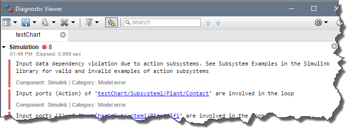
If you ever tried modeling such system, you very likely ran into errors like the following one at some point. The reason is that the Stateflow logic needs the output of the continuous system, and the continuous systems are controlled by the Stateflow chart, creating a loop.

As you will see in the following example, with Simulink subsystems as state, we are now able to pull the continuous algorithm modeled with blocks inside Stateflow, avoiding all those data dependency challenges
Simulink Subsystems as States
To demonstrate this feature, I decided to model a box on a plate moving up and down. When the plate is moving slow, the box and the plate move together as one. If the plate moves fast, the box might leave the plate, free falling in the air.
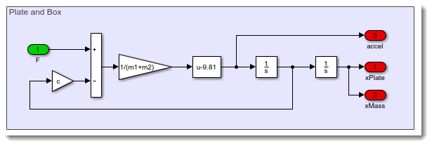
In the first case, the system dynamics can be modeled as:

In the second case, this looks like:

To include those two subsystems in Stateflow, I add two Simulink State and paste the subsystems shown above in each of them. The Inport and Outport blocks of the subsystems will automatically become the inputs and outputs of the Stateflow chart.

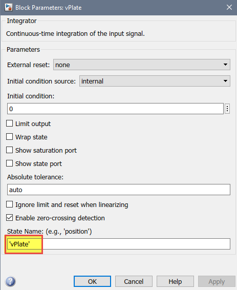
Then I need to name the state of each Integrator block. Those names will be used in the next step to transfer the state when switching mode.

Once this is done, I can define the logic to switch between these two modes.
When the acceleration is larger than gravity in the negative direction, the box will start flying. On the opposite direction, if the box falls and its position becomes smaller or equal to the plate, it lands and begin to move with the plate again. To define those transitions, I can use the inputs and outputs of the chart, and the states explicitly named as described above.
Every time the switching happens, we transfer the states so that the Integrator blocks in the activated subsystem gets initialized with the last values of the Integrator blocks in the subsystem being deactivated.

And that's it, as simple as that! Without the Simulink subsystem as state, modeling this system would have taken a lot more blocks and wiring.
I can now use a PID controller to control the motion of the plate.

If I apply a sinusoidal motion with a high frequency, results show the box jumping on the plate:

Now it's your turn
To see how Simulink subsystems as state can affect the modeling semantics, I recommend comparing the clutch example in R2017a and R2017b. This should make it obvious how this feature simplifies the semantics.
Give this a try and let us know what you think in the comments below.
- カテゴリ:
- Modeling,
- Stateflow,
- What's new?


コメント
コメントを残すには、ここ をクリックして MathWorks アカウントにサインインするか新しい MathWorks アカウントを作成します。