
What is President Trump tweeting about that gets our attention?
Today I'd like to introduce a guest blogger, Grace Kennedy, who works for the Training Services team here at MathWorks. She has been interested in learning what we can find from Twitter, and she will share techniques she uses in her Twitter data analysis.
 Hi, I’m Grace Kennedy. I've been fascinated with how President Trump uses Twitter - what he talks about and how people respond to him. So when the Text Analytics Toolbox was introduced in R2017b, I could not wait to use it to work with Twitter data. In this blogpost, I'll show you how to retrieve and work with tweets and investigate what President Trump is tweeting about that is so popular.
 It turns out that the number of retweets and number of likes are highly correlated, so we can remove the number of retweets. In R2018a, functionality to work more easily with table variables was added, including the removevars function.
 After about five months of data collection, I realized that I had introduced systematic bias into my data. Tweets that are up longer have had more time to collect likes. While the Twittersphere moves quickly, I observed that weekend posts were getting a lot more likes than weekday ones. This was in part because I collected data several times a day... during the workday. This meant weekend tweets would naturally have more time to accumulate likes.
Luckily, I had been stashing my raw data from each pull for reproducibility, so I was able to go back and correct this. I merged datasets, keeping likes from the latest recording available. This is not perfect, but each tweet had a few days to collect likes.
After adjusting for the bias, we test for statistical significance using ttest2 and still see weekend tweets receive more likes than workday tweets. Perhaps this is because people have more time during the weekend to be active on social media.
After about five months of data collection, I realized that I had introduced systematic bias into my data. Tweets that are up longer have had more time to collect likes. While the Twittersphere moves quickly, I observed that weekend posts were getting a lot more likes than weekday ones. This was in part because I collected data several times a day... during the workday. This meant weekend tweets would naturally have more time to accumulate likes.
Luckily, I had been stashing my raw data from each pull for reproducibility, so I was able to go back and correct this. I merged datasets, keeping likes from the latest recording available. This is not perfect, but each tweet had a few days to collect likes.
After adjusting for the bias, we test for statistical significance using ttest2 and still see weekend tweets receive more likes than workday tweets. Perhaps this is because people have more time during the weekend to be active on social media.

 Not only does looking at the hashtags give us an idea of what President Trump is tweeting about (#taxreform, #fakenews, #maga), but we see some abbreviations that represent common phrases he likes to use. I used the custom function below, replaceHashtags, to replace non-word hashtags with their complete phrases (like "MAGA" with his campaign slogan, "Make America Great Again") before visualizing common phrases.

 In the word cloud below, the most popular topic looks like a collection of subjects that includes the FBI investigation and Hillary Clinton. The next three most popular topics are clearer: NFL players kneeling during the national anthem, fake news, and tweets about North Korea.
 Now let's create word clouds for the four least popular topics defined by the fitlda function. As we see in the first word cloud below, the topic that received the fewest number of likes included tweets about something being a great honor to President Trump. Some of the "great honors" were to sign bills into law, meet foreign dignitaries, and visit military sites. These tweets weren't exactly controversial and didn't attract as much attention.
The second least popular topic included tweets about Hurricane Maria, which could be because people are hesitant to click "like" on a tragedy.
Interestingly, it appears President Trump's Twitter followers weren't particularly excited about tweets on the tax overhaul, as we see in the last two word clouds. The third and fourth least popular topics were on this signature legislation, with tweets in the third least popular topic containing more partisan language (dems, republican, party...).
Now let's create word clouds for the four least popular topics defined by the fitlda function. As we see in the first word cloud below, the topic that received the fewest number of likes included tweets about something being a great honor to President Trump. Some of the "great honors" were to sign bills into law, meet foreign dignitaries, and visit military sites. These tweets weren't exactly controversial and didn't attract as much attention.
The second least popular topic included tweets about Hurricane Maria, which could be because people are hesitant to click "like" on a tragedy.
Interestingly, it appears President Trump's Twitter followers weren't particularly excited about tweets on the tax overhaul, as we see in the last two word clouds. The third and fourth least popular topics were on this signature legislation, with tweets in the third least popular topic containing more partisan language (dems, republican, party...).

Hi, I’m Grace Kennedy. I've been fascinated with how President Trump uses Twitter - what he talks about and how people respond to him. So when the Text Analytics Toolbox was introduced in R2017b, I could not wait to use it to work with Twitter data. In this blogpost, I'll show you how to retrieve and work with tweets and investigate what President Trump is tweeting about that is so popular.
Contents
Getting Twitter Data
As of R2017b, you can use MATLAB functions from the Datafeed Toolbox to retrieve tweets. First you will need to sign up for a developer account with Twitter to obtain credentials. I have my developer credentials saved as a MAT-file for privacy. We pass our credentials to the twitter function to open a connection to the Twitter API. Then, searching Twitter is an easy one-liner with the search function. The response is a struct with information about the individual tweets and the search metadata.load creds.mat connection = twitter(consumerKey,consumerSecret,accessToken,accessTokenSecret); % 100 is the maximum number of tweets that can be pulled at a time response = search(connection,'mathworks','count',100,'lang','en')
response =
  ResponseMessage with properties:

    StatusLine: 'HTTP/1.1 200 OK'
    StatusCode: OK
        Header: [1×26 matlab.net.http.HeaderField]
          Body: [1×1 matlab.net.http.MessageBody]
     Completed: 0
Each status contains information about a single tweet, such as the number of likes, when the tweet was posted, and the text of the tweet.
% extract each status as a string
tweets = cellfun(@(x) extractBefore(string(x.text),50), response.Body.Data.statuses);
tweets(1:3)
ans =
  3×1 string array
    "listening to NPR and there's a mathworks ad? :thi"
    "RT @MetrowestSTEM: Thank you @MathWorks, Underwri"
    "Basics of eigenvalues and eigenvectors with MIT P"
I was looking for tweets from a specific user. The syntax for queries that are more advanced than just a search string can be found in the Twitter documentation. This query takes the form 'from:mathworks'. However, we must use percent encoding. So, we need to change the colon to %3A. We can automate percent encoding using a trick from Toshi Takeuchi's February blogpost, which sparked my original interest in using MATLAB for Twitter analysis.
pctencode = @(str) replace(char(java.net.URLEncoder.encode(str,'UTF-8') ),'+','%20');
st = pctencode('from:mathworks')
st =
    'from%3Amathworks'
response = search(connection,st,'count',100,'lang','en');
tweets = cellfun(@(x) extractBefore(string(x.text),50), response.Body.Data.statuses);
tweets(1:3)
ans =
  3×1 string array
    "#HardTech Is it possible to add EtherCAT Master t"
    "Uses #drones and kites as #renewable energy sourc"
    "Are We Taking the “U” Out of UX? - What is a UX d"
Several months and 1033 tweets later, here is what I found.
There Was More to Defining Popularity Than I Expected
My first thought was to define popularity as the number of retweets and likes a tweet receives. So, as I pulled Twitter responses, I saved these metrics, the date of each tweet, and the tweets themselves.data = readtable('someTrumpTweets.csv','TextType','string'); data = table2timetable(data);Let's take a quick peek at the numeric data.
subplot(2,1,1)
plot(data.whenTweeted,[data.retweetsNo,data.likesNo],'o')
legend('Number of Retweets', 'Number of Likes', 'Location','northwest')
axis('tight')
subplot(2,1,2)
plot(data.retweetsNo,data.likesNo,'o')
xlabel('Number of Retweets')
ylabel('Number of Likes')
It turns out that the number of retweets and number of likes are highly correlated, so we can remove the number of retweets. In R2018a, functionality to work more easily with table variables was added, including the removevars function.
data = removevars(data,'retweetsNo');
I also looked at whether the time of day or day of the week had any effect on the popularity of a tweet. This was easy with the groupsummary function in R2018a, which enables group summary statistics on timetables. While I didn't find that popularity of the tweets varied by time of day, I did find that President Trump tweets more at some times than others.
% number of tweets by hour of day
byHour = groupsummary(data(:,'likesNo'),'whenTweeted','hourofday');
figure
bar(0:23,byHour.GroupCount)
xlabel('Hour of the Day')
ylabel('Total Number of Tweets')
title('Number of Tweets By Hour of the Day')
After about five months of data collection, I realized that I had introduced systematic bias into my data. Tweets that are up longer have had more time to collect likes. While the Twittersphere moves quickly, I observed that weekend posts were getting a lot more likes than weekday ones. This was in part because I collected data several times a day... during the workday. This meant weekend tweets would naturally have more time to accumulate likes.
Luckily, I had been stashing my raw data from each pull for reproducibility, so I was able to go back and correct this. I merged datasets, keeping likes from the latest recording available. This is not perfect, but each tweet had a few days to collect likes.
After adjusting for the bias, we test for statistical significance using ttest2 and still see weekend tweets receive more likes than workday tweets. Perhaps this is because people have more time during the weekend to be active on social media.
data.wkEnd = isweekend(data.whenTweeted);
boxplot(data.likesNo,data.wkEnd,'Labels',{'Weekday' 'Weekend'})
ylabel('Number of Likes')
title('Weekday vs. Weekend')
% test for statistical significance
ttest2(data.likesNo(data.wkEnd),data.likesNo(~data.wkEnd))
ans =
     1
What are all the tweets about?
The president likes to call out individuals, themes, and slogans with hashtags and @ mentions. It is a concise way of linking ideas and people or corporations. As of R2018a, we can identify many of these common elements in text data with the 'DetectPatterns' option for the tokenizedDocument function. Hashtags give us a pretty good idea of what President Trump likes to call out.tweetDocuments = tokenizedDocument(data.tweets,'DetectPatterns',{'at-mention','hashtag','web-address'}); tweetDeets = tokenDetails(tweetDocuments); tweetDeets(37:39,:)
ans =
  3×4 table
     Token      DocumentNumber    LineNumber       Type
    ________    ______________    __________    ___________
    "Jersey"          2               1         letters
    "."               2               1         punctuation
    "#MAGA"           2               1         hashtag
hashtags = tweetDeets(tweetDeets.Type == 'hashtag',:);
wordcloud(hashtags.Token);
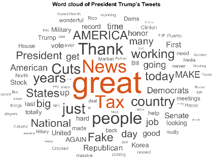
Not only does looking at the hashtags give us an idea of what President Trump is tweeting about (#taxreform, #fakenews, #maga), but we see some abbreviations that represent common phrases he likes to use. I used the custom function below, replaceHashtags, to replace non-word hashtags with their complete phrases (like "MAGA" with his campaign slogan, "Make America Great Again") before visualizing common phrases.
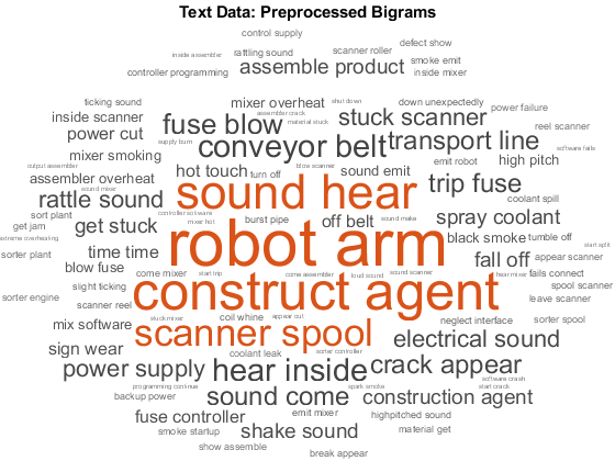
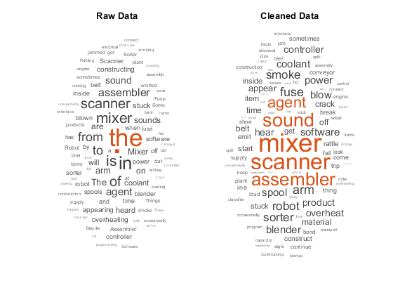
% make everything lower case
cleanDocs = lower(tweetDocuments);
% replace hashtag abbreviations with standard language
cleanDocs = replaceHashtags(cleanDocs);
As of R2018a, we can create bags of N-grams, which enables us to look at phrases rather than just individual words. I first did a little processing to remove some noise in the form of punctuation or words that don't tell us much about the content.
% erase punctuation
cleanDocs = erasePunctuation(cleanDocs);
% remove common words before analysis
cleanDocs = removeWords(cleanDocs,stopWords);
% remove two letter words
cleanDocs = removeShortWords(cleanDocs,2);

bag = bagOfNgrams(cleanDocs,'NgramLengths',3);
w = wordcloud(bag);
And which topics are the most popular?
We can sort the tweets into a set number of previously undetermined topics using the fitlda function from the Text Analytics Toolbox. I chose eighteen as the number of topics using the perplexity metric in the LDA model. For more details, please refer to this example.bag2Model = bagOfWords(cleanDocs); % set seed for reproducibility rng(123) numTopics = 18; mdl = fitlda(bag2Model,numTopics,'Verbose',0); [~,topics] = max(mdl.DocumentTopicProbabilities,[],2); data.topics = topics;Not every tweet fits perfectly into one of eighteen well-defined topics. To help me label the topics, I removed some of the noise by excluding tweets classified with the lowest confidence.
p = mdl.DocumentTopicProbabilities; maxs = max(p,[],2); cutoff =...
quantile(maxs,.5); dataTrimmed = data(maxs>=cutoff,:);
for ii = 1:numTopics
     figure wordcloud(dataTrimmed.tweets(dataTrimmed.topics == ii));
end
Finally, let's get the average number of likes by topic so we can look at the four most and least popular topics.
popCats = groupsummary(data(:,{'likesNo','topics'}),'topics','mean');
load topicNames.mat

bar(topicNames, popCats.mean_likesNo);
title('Popularity by Topics')
ylabel('Number of Likes')
In the word cloud below, the most popular topic looks like a collection of subjects that includes the FBI investigation and Hillary Clinton. The next three most popular topics are clearer: NFL players kneeling during the national anthem, fake news, and tweets about North Korea.
[~,idx] = sort(popCats.mean_likesNo,'descend');

rank = ["The" "Second" "Third" "Fourth"];
nGrams = [1 2 1 2];
for ii = 1:4
    subplot(2,2,ii)
    bag = bagOfNgrams(cleanDocs(data.topics == idx(ii)),'NgramLengths',nGrams(ii));
    wordcloud(bag);
    text = rank(ii) + " Most Popular, N-Grams = " + nGrams(ii);
    title(text)
end
Now let's create word clouds for the four least popular topics defined by the fitlda function. As we see in the first word cloud below, the topic that received the fewest number of likes included tweets about something being a great honor to President Trump. Some of the "great honors" were to sign bills into law, meet foreign dignitaries, and visit military sites. These tweets weren't exactly controversial and didn't attract as much attention.
The second least popular topic included tweets about Hurricane Maria, which could be because people are hesitant to click "like" on a tragedy.
Interestingly, it appears President Trump's Twitter followers weren't particularly excited about tweets on the tax overhaul, as we see in the last two word clouds. The third and fourth least popular topics were on this signature legislation, with tweets in the third least popular topic containing more partisan language (dems, republican, party...).
nGrams = [2 2 1 2];
for ii = 0:3
    subplot(2,2,ii+1)
    bag = bagOfNgrams(cleanDocs(data.topics == idx(end-ii)),'NgramLengths',nGrams(ii+1));
    wordcloud(bag);
    text = rank(ii+1) + " Least Popular with N-Grams = " + nGrams(ii+1);
    title(text)
end
Do you work with text data?
I've enjoyed watching my word clouds change daily with the speed of the news, and now, stepping back to analyze the popularity of various topics. I am wondering who else uses MATLAB to work with Twitter data. What are you investigating? What methods do you use to retrieve and analyze data? More generally, what kinds of text data do you come across in your work or hobbies? What insight could topic modeling provide? Let us know here!function cleanTweets = replaceHashtags(tweets) % custom function used in "What are all the tweets about?" to replace % hashtags with full expressions cleanTweets = tweets; oldFN = "fakenews"; newFN = "fake news"; cleanTweets = replace(cleanTweets,oldFN,newFN); oldHH = string({"hurricaneharvey"}); newHH = "hurricane harvey"; cleanTweets = replace(cleanTweets,oldHH,newHH); oldNK = string({"northkorea" "noko"}); newNK = "north korea"; cleanTweets = replace(cleanTweets,oldNK,newNK); oldTR = string({"taxreform"}); newTR = "tax reform"; cleanTweets = replace(cleanTweets,oldTR,newTR); oldPR = string({"puerto rico"}); newPR = "puerto rico"; cleanTweets = replace(cleanTweets,oldPR,newPR); oldPRs = string({"prstrong"}); newPRs = "puerto rico strong"; cleanTweets = replace(cleanTweets,oldPRs,newPRs); oldStand = string({"standforouranthem"}); newStand = "stand for our anthem"; cleanTweets = replace(cleanTweets,oldStand,newStand); oldMAGA = string({"maga"}); newMAGA = "make america great again"; cleanTweets = replace(cleanTweets,oldMAGA,newMAGA); oldAF = string({"americafirst"}); newAF = "america first"; cleanTweets = replace(cleanTweets,oldAF,newAF); oldTC = string({"taxcutsandjobsact"}); newTC = "tax cuts and jobs act"; cleanTweets = replace(cleanTweets,oldTC,newTC); endPublished with MATLAB® R2018a
- Category:
- New Feature,
- Strings


Comments
To leave a comment, please click here to sign in to your MathWorks Account or create a new one.