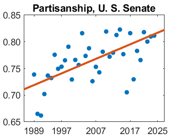
My first blog about SVD and Partisanship in the U. S. Senate was five years ago. Today's post updates that to 2025.... read more >>

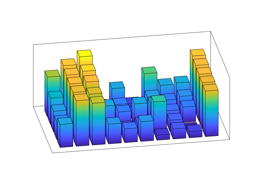
I admire the color scheme in the New York Times Games section and occasionally make it my colororder.... read more >>

Rob Schrieber is one of my very best friends.... read more >>

Nick Trethen is a world famous computational scientist and my good friend.... read more >>

Jack Dongarra is my student, colleague and friend.... read more >>

Pete Stewart is one of my closest colleagues.... read more >>

The tangram is an ancient Chinese puzzle with seven pieces.... read more >>

I was invited recently to give a virtual talk to the student chapter of SIAM at JUIT, the Jaycee Institute of Information Technology, in Wagnaghat, India.... read more >>

Like millions of other folks, I play Wordle from the New York Times almost every day. The Times reports that Wordle puzzle number 1497 on Friday, July 25, was especially difficult. The average puzzler required 5.7 attempts and many failed to get the answer in the six moves allowed. I have a MATLAB assistant that I call Wordler and, even with her help, I failed on number 1497. Here's why.... read more >>

In 1988, while I was with Ardent Computer in Silicon Valley, I gave a talk that previewed MATLAB graphics. The title was "Pictures of Matrices". At the time, a mathematician friend of mine asked.... read more >>