
Optimizing to Survive
Today's guest blogger is Mary Fenelon, who is the product marketing manager for Optimization and Math here at MathWorks. In today's post she describes how she uses optimization to try to best the rest of the product marketing team.
The National Football League 2018 season will soon be_ (is?)_ upon us. Several of us in the product marketing team here at MathWorks have played in an office league for the last couple of years. I don't follow the NFL very closely so I didn't think about participating until one of my fellow product marketing managers challenged me to do so by remarking that this looked like an optimization problem. That's all it took!
Contents
Rules
- This is a knockout or survivor style pool. Every week, your goal is to pick the winning team for one game. You can only choose a team once for the entire season. If your team wins or ties you move on to the next week and pick from the remaining teams. As long as you haven’t picked a losing team you can choose from the entire group of NFL teams.
- If you pick a losing team you are not out of the knockout pool. You are now restricted to picking from the teams that had a non-winning record last season. You can try to keep your streak alive, but now you have to do it with a more limited set of teams.
- Whoever is alive for the longest number of weeks wins the knockout pool. The longer you keep the knockout streak alive the bigger the knockout pool grows. It will start at 50% of the pool, and grow onward. The pot will grow until the last person has two losses. If two or more people tie, they will either split the pool or determine a final winner by a joust in the parking lot.
- After your second loss you can still win the secondary pool, which is whoever picks the most winners throughout the season. Once you’ve lost twice you can go back to picking any team as long as you haven’t already picked them. Whoever wins the knockout pool is ineligible for this prize unless there’s unforeseen circumstances (if everyone is knocked out in week 2, for example).
My Strategy
I could choose a team each week without considering that it would be better to choose that team further out. That myopic strategy could leave me with poor choices at the end of the season. Instead, my first strategy decision is to run an optimization each week choosing teams for all of the remaining weeks of the season but use only the choice for the current week. That way, I benefit from updated information as the season progresses while still looking at the whole schedule.
Coming up with a set of choices can be modeled as a linear assignment problem. The goal in an assignment problem is to assign workers to tasks so that the cost of completing all the tasks is minimized. Each worker can only do one task. For the NFL pool, the workers are the teams and the tasks are the weeks.
What to use for the costs of each team-to-week assignment? This choice is the second place where the art and science of modeling comes into play. Art, to think of measures, and science, to validate that the chosen measure gives the desired result. My choice is to use the win probabilities produced by fivethirtyeight.com. This article explains how they built their predictive model using the entire history of the NFL as data. With that measure, the objective is to maximize the sum of the win probabilities of the chosen teams over the entire season.
Linear assignment problems can by solved by the Hungarian algorithm. This implementation on the MATLAB File Exchange is a popular one. These problems can also be solved by the functions in Optimization Toolbox. Formulating the problem as an optimization problem gives me the option to specify additional constraints, for instance, to follow the rule that after one loss, I'm restricted to choose from the losers bracket.
Data
Season Data
For this post, I'll generate some data instead of using actual NFL data. I'll use about half the teams and half as many games as the NFL.
nSeasonWeeks = 8;
teams = ["Aardvarks","Bats","Cheetahs","Dragons","Emus","Foxes","Giraffes","Hippos","Ibexes","Jackals",...
    "Koalas","Lemurs","Monkeys","Newts","Otters","Porcupines"]';
nTeams = numel(teams);
Designate some teams as losers from the previous season for the losers bracket. Set the random seed to reproduce the same bracket each time I run the script.
rng(19);
nLosers = floor(nTeams/2);
idx = randperm(nTeams);
losers = teams(idx(1:nLosers));
Weekly Data
I'll rerun the model each week, keeping track of the week of the season and which teams I already picked.
Each week I increment the week counter.
thisWeek = 2;
Each week I add the team that was chosen the previous week
previousPicks = ["Aardvarks"];
Generate the labels for the remaining weeks:
weeks = "week" + string(thisWeek:nSeasonWeeks)';
nWeeksLeft = nSeasonWeeks - thisWeek + 1;
Get the probabilities.
Here's where I would scrape a web page for predictions. Instead, I'll use a random matrix for the win probabiliites. The random values won't show the patterns one would see in real data, but they are sufficient for showing how to set up and run the optimization model. One step towards more realistic probabilities is to first generate team pairings for the games and a game schedule. This is an optimization problem in itself; for an example see scheduling the ACC basketball conference.
winProbs = rand(nTeams,nWeeksLeft);
Linear Assignment Model
I will use the problem-based workflow for optimization introduced in R2017b. This workflow simplifies the process of specifying and solving linear and mixed-integer linear programs, that is, optimization problems with linear constraints and objectives and with variables that can take on continuous or discrete values.
Variables
First, define a two dimensional optimvar, x, indexed by teams and weeks. The optimization solver will compute values for an optimvar include in an optimproblem. I make this a binary variable, that is a variable that only takes on the values of 0 and 1 with this statement:
x = optimvar('x',teams,weeks,'LowerBound',0,'UpperBound',1,'Type','integer');
In my model, a value of 1 for x(i,j) will mean that team i is chosen for week j and a value of 0 means it is not chosen.
To eliminate a team that's already been picked, set the upper bounds of variables corresponding to those teams to 0.
x.UpperBound(previousPicks,weeks) = 0;
Optimization Problem and Objective
Next, define the optimization problem and the objective to maximize the sum of the win probabilities of the chosen teams:
p = optimproblem;
p.ObjectiveSense = 'maximize';
p.Objective = sum(sum(winProbs.*x));
Constraints
The first constraint statement generates one constraint for each team: a team can be chosen at most once. The result is an optimconstr. Show the first constraint of each set to check the formulation as it's built.
p.Constraints.eachTeamAtMostOnce = sum(x,2) <= 1;
showconstr(p.Constraints.eachTeamAtMostOnce(1))
  x('Aardvarks', 'week2') + x('Aardvarks', 'week3')
+ x('Aardvarks', 'week4') + x('Aardvarks', 'week5')
+ x('Aardvarks', 'week6') + x('Aardvarks', 'week7')
+ x('Aardvarks', 'week8') <= 1
The second constraint statement generates one constraint for each week: a team must be choosen.
p.Constraints.mustPickOne = sum(x,1) == 1;
showconstr(p.Constraints.mustPickOne(1))
  x('Aardvarks', 'week2') + x('Bats', 'week2') + x('Cheetahs', 'week2')
+ x('Dragons', 'week2') + x('Emus', 'week2') + x('Foxes', 'week2')
+ x('Giraffes', 'week2') + x('Hippos', 'week2') + x('Ibexes', 'week2')
+ x('Jackals', 'week2') + x('Koalas', 'week2') + x('Lemurs', 'week2')
+ x('Monkeys', 'week2') + x('Newts', 'week2') + x('Otters', 'week2')
+ x('Porcupines', 'week2') == 1
Solve
Now solve the optimization problem. The solve function will call the mixed-integer linear programming solver, intlinprog,| b|ecause some of the optimization variables are of type integer
soln = solve(p);
LP:                Optimal objective value is -6.661074.


Optimal solution found.

Intlinprog stopped at the root node because the objective value is within a gap
tolerance of the optimal value, options.AbsoluteGapTolerance = 0 (the default
value). The intcon variables are integer within tolerance,
options.IntegerTolerance = 1e-05 (the default value).
Tabulate choices
Optimization Toolbox solvers use floating point arithmetic so it's possible that the solution values may not be integral. I want to use the values as logical indexes, so I will round them just to be sure that they are.
picks = round(soln.x);
[teampicks,weekpicks] = find(picks);
probpicks = find(picks);
table(weeks(weekpicks),teams(teampicks),winProbs(probpicks),...
     'VariableNames',{'Week','Team','WinProb'})
ans =
  7×3 table
     Week        Team       WinProb
    _______    _________    _______
    "week2"    "Foxes"      0.94616
    "week3"    "Lemurs"      0.9943
    "week4"    "Bats"       0.97137
    "week5"    "Koalas"     0.99744
    "week6"    "Dragons"    0.91183
    "week7"    "Ibexes"     0.98344
    "week8"    "Hippos"     0.85654
Extending the Model
The win probabilities will be updated on the results of the prior games as the season progresses. Maybe I don't want to value the probabilities for the end of the season as highly as those in the current week. This can be done by applying a discount factor. In the Live Script version of this post, I set the discount factor with a Live Control to make it easy to experiment with different values.
discountFactor =0.05
scalePerWeek = (1-discountFactor).^(0:nWeeksLeft-1);
dProbs = winProbs.*scalePerWeek;
p.Objective = sum(sum(x.*dProbs));
soln = solve(p);
[teampicks,weekpicks] = find(picks);
probpicks = find(picks);
table(weeks(weekpicks),teams(teampicks),winProbs(probpicks),...
     'VariableNames',{'Week','Team','WinProb'})
discountFactor =
         0.05
LP:                Optimal objective value is -5.755877.


Optimal solution found.

Intlinprog stopped at the root node because the objective value is within a gap
tolerance of the optimal value, options.AbsoluteGapTolerance = 0 (the default
value). The intcon variables are integer within tolerance,
options.IntegerTolerance = 1e-05 (the default value).

ans =
  7×3 table
     Week        Team       WinProb
    _______    _________    _______
    "week2"    "Foxes"      0.94616
    "week3"    "Lemurs"      0.9943
    "week4"    "Bats"       0.97137
    "week5"    "Koalas"     0.99744
    "week6"    "Dragons"    0.91183
    "week7"    "Ibexes"     0.98344
    "week8"    "Hippos"     0.85654
Applying a discount factor of 5% didn't change the results.
I might want to only choose winning teams when I have no losses so that I can pick the best of the losing teams when I have to pick among them.
onlyWinners = false;
if onlyWinners
    p.Constraints.onlyWinners = sum(x(losers,weeks),1) == 0;

end
With one loss, I must pick from the losers bracket.
onlyLosers = true;
if onlyLosers
    p.Constraints.onlyLosers = sum(x(losers,weeks),1) >= 1;
    showconstr(p.Constraints.onlyLosers(1))
end
  x('Aardvarks', 'week2') + x('Cheetahs', 'week2') + x('Dragons', 'week2')
+ x('Emus', 'week2') + x('Foxes', 'week2') + x('Koalas', 'week2')
+ x('Newts', 'week2') + x('Otters', 'week2') >= 1
soln = solve(p);
[teampicks,weekpicks] = find(picks);
probpicks = find(picks);
table(weeks(weekpicks),teams(teampicks),winProbs(probpicks),...
     'VariableNames',{'Week','Team','WinProb'})
LP:                Optimal objective value is -4.838951.


Optimal solution found.

Intlinprog stopped at the root node because the objective value is within a gap
tolerance of the optimal value, options.AbsoluteGapTolerance = 0 (the default
value). The intcon variables are integer within tolerance,
options.IntegerTolerance = 1e-05 (the default value).

ans =
  7×3 table
     Week        Team       WinProb
    _______    _________    _______
    "week2"    "Foxes"      0.94616
    "week3"    "Lemurs"      0.9943
    "week4"    "Bats"       0.97137
    "week5"    "Koalas"     0.99744
    "week6"    "Dragons"    0.91183
    "week7"    "Ibexes"     0.98344
    "week8"    "Hippos"     0.85654
Results
So how did I do? In both years, I was knocked out fairly early but finished at the top of the secondary pool.
Unfortunately, one player had no losses in both years so there was no secondary pool award. That player has not revealed his strategy but there is speculation that he uses an optimization model. A player with just one loss did reveal his strategy: picking the best team from fivethirtyeight.com each week. That's the myopic strategy I didn't want to use! I can see why it makes sense, though. There are about twice as many teams as games so as long as you can pick from the entire league, there should be some good picks available each week. A greedy strategy also makes sense when the predictions are changing during the season.
I'm not willing to give up on placing well in the secondary pool so I'll keep my assignment model. I can make it greedier by using a higher discount factor. Maybe I should also deal with the uncertainty in the probabilities by using data from more than one source or by using a stochastic optimization approach. Now that I have two years worth of data I can do some model validation before deciding on this year's strategy. It's time to get busy!
Do you have a better approach? Let us know your thoughts here.
- Category:
- Optimization


Comments
To leave a comment, please click here to sign in to your MathWorks Account or create a new one.