
Deep Learning Tutorial Series
Our guest post this week is written by Johanna: her pick of the week is a new Deep Learning Tutorial Series. This post is going to introduce the tutorial, a new video series on deep learning, and a lot of other links to get started with deep learning. Enjoy!
Avi wrote about deep learning in 11 lines of code. If you’re just starting out in deep learning, I encourage you to go there first: it’s a great post and a great way to get started. But let’s go a bit further. What happens if we want to create our own network to identify new objects in images?
The entry on File Exchange is going to provide you with 3 examples:
- Training a neural network from scratch
- Transfer learning
- Using a neural network as a feature extractor
These three examples are intended to help you create a custom neural network for your data. Also, they are less than 125 lines of code… total!
The examples were built using images from CIFAR-10, a publicly available database of relatively small [32 by 32 pixels] images. There is a file included called DownloadCIFAR10.m that will download the images and place them into a test and training folder. It will take some time to download and extract these images, but you only need to run this once.
If you aren’t ready to dive into code just yet, or if you would like an overview of deep learning, check out our introductory video series on neural networks. This will help answer these questions:
• What is deep learning?
• What is a neural network?
• What’s the difference between machine learning and deep learning?
Deep Learning Introductory Series
All the examples require large sets of image data. If you are new to MATLAB and you have lots of data – image data or other – please check out ImageDatastore which is built on Datastore to better manage large amounts of data.
Training a neural network from scratch
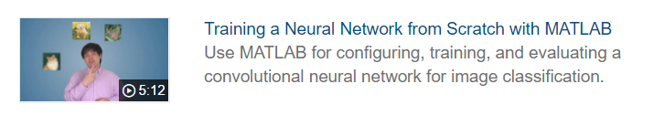
We’ll jump right into creating a neural network from scratch that can identify 4 categories of objects. Sounds intimidating? A neural network is simply a series of layers that each alter the input and pass the output to the next layer. This figure helps visualize the process.

Want to understand CNNs at a deeper level? Check out this short video where we dive into the key aspects of ConvNets.
 |
 |
The code will give you a pre-defined neural network to start with, but the concept of creating a network from scratch means you have the freedom to explore the architecture and alter it as you see fit. This is an opportunity to take this example network see how changing the layers affects the accuracy. Running the code in the example without any alterations – you will see the accuracy is around 75%. Can you find a way to increase the accuracy further?
Transfer Learning
![]()
Transfer learning is this semi-bizarre notion that you can take someone else’s fully baked network and transfer all the learning it has done to learn a completely new set of objects. If a network has been fed millions of images of dogs and cats – and can accurately predict those categories – it may only take a few hundred images to learn a new category like rabbits. The learning can be transferred to new categories. Like the video explains, it helps if your new recognition task is similar or has similar features to the original categories. For example, a network trained on dogs may be well suited to learn other animals relatively quickly.
It also helps to have an accurate network to start with, which is why we’ll start our example using AlexNet, a ConvNet that won the 2012 ILSVRC competition. It has been trained on many kinds of animals, and since we want to identify dogs, frogs, cats and deer, we expect this network to be a great starting point.
Importing AlexNet is a breeze in MATLAB
net = alexnet;
If this is your first time running this code, you may get an error message. Follow the link to download AlexNet. You only need to download AlexNet once.
Let’s look at the last few layers of the network. You’ll see AlexNet was trained for 1000 different categories of objects.
layers = net.Layers
…

23   'fc8'      Fully Connected               1000 fully connected layer

24   'prob'     Softmax                       softmax

25   'output'   Classification Output         crossentropyex with 'tench', 'goldfish', and 998 other classes
As a quick aside, if you want to see all 1000 categories that AlexNet is trained on, here’s a fun line of code:
class_names = net.Layers(end).ClassNames;
Back to the demo. Notice layer 23, where it says 1000 fully connected layer? We’ll need to change that 1000 to 4, since we have four categories of objects.
Take layers from AlexNet, then add our own
layers = layers(1:end-3);

 layers(end+1) = fullyConnectedLayer(4, 'Name', 'fc8_2 ');

 layers(end+1) = softmaxLayer;

 layers(end+1) = classificationLayer()
After we alter the network, we can quickly* re-train it
convnet = trainNetwork(imds, layers, opts);
*Quickly is a relative term depends on your hardware and number of training images.
At the very end, we have a custom network to recognize our four categories of objects:
 |
 |
 |
 |
How well does it do? Running this script gave me an accuracy of roughly 80%. Of course, this is a random process, so you can expect slight variations in this number. Can you get a much higher accuracy on these four categories? Leave a comment below!
Feature Extraction
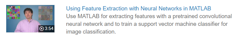
Perhaps a less common technique of neural networks is using them as feature extractors. What does that mean exactly? Gabriel explains the concepts of features and feature extraction very well in the video above.
The accuracy of neural networks is due in part to the huge amount of data used to train them. In fact, AlexNet – the network used as a starting point for the second and third example – was trained on millions of images. You can expect that the lower layers of the network can identify rich features that define the individual objects, so what happens if we simply extract these features?
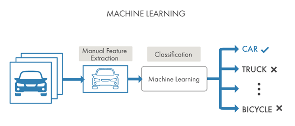
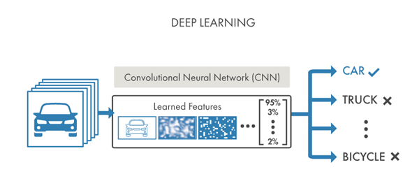
Here, we have a typical machine learning and deep learning workflow. Let’s combine these workflows and make a super-classifier*!
*Super-classifier isn’t a technical term.

Using a CNN as a feature extraction technique, and then using those features in a machine learning model can be a highly versatile use of deep learning.
Notice how easy MATLAB makes extracting these features from a test set.
featureLayer = 'fc7';

trainingFeatures = activations(convnet, trainingSet, featureLayer);
 |
 |
The features can be extracted from any place in the network. We choose the last fully connected layer these will be the most complex and descriptive for our categories, but you could choose the features at an earlier stage. What if you choose features from another layer? How does this affect the accuracy? You can even visualize the activations of the network in this example.
Another benefit of using a feature extraction approach is the ability to choose whichever classifier will best fit the data. We’re using a multi-class svm in the video:
fitcecoc
We could also choose a multi-class naive Bayes model – fitcnb – or a k-nearest neighbor classification model – fitcknn – or a variety of other classification models.
It’s great to have to many options, but how on earth do you know which classifier to choose?
Check out our classification learner app to find the best model for the data.
Another advantage to feature extraction using ConvNets is you need much less data to get an accurate result. At the very end of the demo, we see that with minimal data, we get an accuracy of approximately 77%. We intentionally used less data [50 images per category] in this example to show how you can still use a deep learning approach without thousands of sample images. Would increasing the number of training images also increase the accuracy?
Take the code at line number 11
[trainingSet, ~] = splitEachLabel(imds, 50, 'randomize');
and change the number 50 to a higher number to increase the number of samples per category.
Summary
These three examples and corresponding videos can help you explore 3 different ways of creating a custom object recognition model using deep learning techniques.
Give it a try and let us know what you think here or leave a comment for the Deep Learning Team.
- Category:
- Picks


Comments
To leave a comment, please click here to sign in to your MathWorks Account or create a new one.