
Bouncing Rod Simulator
As a mechanical engineer, I love simulating physical phenomena. When you have equations of motion, you can easily simulate them in MATLAB using ODE solvers. Of course, you can also simulate dynamic systems with Simulink or with our physical modeling tools. With ODE solvers, you can detect events to simulate things like a bouncing ball. (By the way, here's an example of a bouncing ball simulated using Simulink).
When I saw this simulation of a bouncing rod by Matthew, it brought me a smile. This is a nice extension to the bouncing ball simulator:
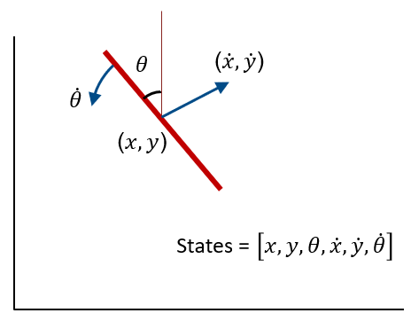
- The rod moves in 2 dimensions. Positional states include $ \left[x, y, \dot{x}, \dot{y}\right] $
- The rod can also rotate. Rotational states include $ \left[\theta, \dot{\theta}\right] $
- Collision (contact) with the ground can happen in multiple cases: top tip of the rod hitting the ground, bottom tip of the rod hitting the ground, or the rod hitting the ground (mostly) parallel to the ground. Based on the situation, the new states for the rod are calculated.
- There are two different modes of operation: flight and sliding. Typically the rod is in flight mode. When the rod reaches a certain state, it eventually switches to sliding mode.
Once the simulation finishes, it shows the animation of the dynamics.

This is a great example to understand the concept of ODE solvers and the event-handling capability of the solvers. This serves the purpose of teaching those concepts. There are, however, a couple of additional effects that could be added to this simulation to make it even more true to the physics.
- Add friction - you can see this especially once the rod goes into sliding mode. The rod keeps sliding forever. Adding frictional forces to slidingPhase.m can accomplish this.
- Improve the switching logic for sliding - currently, the rod switches to sliding mode when it detects that the center of mass (COM) is close to the ground. This logic indicates that when the COM is close to zero, the rod is nearly parallel to the ground. This may be a reasonable logic for most cases. However, it doesn't accurately represent a case where the rod falls down flat on the ground with vertical speed. In reality, the rod will bounce up due to impact, but the simulation switches to sliding in this case. Here's an example of a case where the rod falls parallel to the ground. One approach would be to look at not just the COM but also the vertical speed of the rod. Another approach is to calculate the states after collision, and switch to sliding mode only if the vertical speed is below a threshold.
These are improvement ideas, but they don't take away any of the value this entry provides to people wanting to simulate dynamic systems with event handling.
Comments
- Category:
- Picks


Comments
To leave a comment, please click here to sign in to your MathWorks Account or create a new one.