
Simulations of Brownian particle motion
Today’s post is by Owen Paul, who is a Student Ambassador Technical Program Specialis. He himself was a student ambassador before joining MathWorks, and he was featured in the Community Blog.


Contents
Introduction
This week’s pick is Simulations of Brownian particle motion by Emma Gau. This file exchange entry caught my eye because it is featured on the Live Script gallery and Emma Gau is one of our student ambassadors! She has been a student ambassador for MathWorks for 3 years at UC Santa Barbara.Background
If you were to look at a window with sunlight shining in, you might be able to notice little particles of dust flying around. No matter how hard you try to swat the particles of dust they will continue to float around aimlessly. This phenomenon is described by Brownian motion. Trying to predict where these particles go can be extremely difficult due to the randomness of their motion. In this file exchange entry, Emma shows us how we can use the Euler?Maruyama (EM) method to simulate how the particles move in a 1 dimensional (1D) plane. When asked about what drove Emma to write this live script on such a topic, she said that the “project was created from [her] research on Brownian particle motion while assisting Prof. Atzberger’s (UCSB) work on differentiable manifolds.” But then she adapted the work into this live script to compete in the MATLAB Online Live Editor Challenge hosted in 2018.Main code applying EM method
Now let’s dive into some of the core elements of this live script. In this live script we can see how to apply the EM method for 1D Brownian motion but also the approximate error with this analysis. We can see this plotted below with the blue line representing the actual path and the green dotted line the predicted motion.randn('state',100) lambda = 2; mu = 1; Xnot = 1; T = 1; N = 2^8; dt = 1/N; dW = sqrt(dt)*randn(1,N); W = cumsum(dW); X_exact = Xnot*exp((lambda-.5*mu^2)*([dt:dt:T])+mu*W); plot([0:dt:T],[Xnot,X_exact],'b-'); hold on R = 4; Dt = R*dt; L = N/R; X_EM = zeros(1,L); X_temp = Xnot; for j = 1:L Winc = sum(dW(R*(j-1)+1:R*j)); X_temp = X_temp + Dt*lambda*X_temp + mu*X_temp*Winc; X_EM(j) = X_temp; end plot([0:Dt:T],[Xnot,X_EM],'g--o') hold off xlabel('t'); ylabel('X'); title('Approximation error with 10^4 samples')
Solving Brownian simulation using other methods
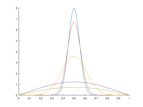
This code also has a bonus as it shows how we would also solve this problem numerically. This directly shows the difference in the approach of tackling the problem but also shows how different it is coding these two methods.numx = 101; numt = 2000; dx = 1/(numx - 1); dt = 0.00005; x = 0:dx:1; C = zeros(numx,numt); t(1) = 0; C(1,1) = 0; C(1,numx) = 0; mu = 0.5; sigma = 0.05; for i=2:numx-1 C(i,1) = exp(-(x(i)-mu)^2/(2*sigma^2)) / sqrt(2*pi*sigma^2); end for j=1:numt t(j+1) = t(j) + dt; for i=2:numx-1 C(i,j+1) = C(i,j) + (dt/dx^2)*(C(i+1,j) - 2*C(i,j) + C(i-1,j)); end end figure hold on plot(x,C(:,1)); plot(x,C(:,11)); plot(x,C(:,101)); plot(x,C(:,1001)); plot(x,C(:,2001)); hold off
Benefits of Live scripts
In this live script not only do we see the code in order to do this analysis, but Emma also takes us through the theory as well (pictured below). I believe this to be one of the most powerful elements in this live script. In the live script Emma shows how the EM method is derived to apply to Brownian motion. Which allows for better understanding of the code. When asked about using a live script for this project she said that,“using live scripts is a great way to compile functions and to share them. It makes it very easy for others to learn from since you can see the code and run it in real time. This was actually my first time experimenting with the live script function in MATLAB for the competition and I think it is definitely something that I would use in the future.”
Comments
Let us know what you think here leave a comment for Emma.- Category:
- Picks


Comments
To leave a comment, please click here to sign in to your MathWorks Account or create a new one.