
Tracing the boundary of a binary region in an image
Brett's Pick this week is Freeman chain code, by Nicolas Douillet.
Contents
A new file prompts a thought experiment
I've never done this before, but I've decided to write about a file that just went live today (as I write this)! I was excited to see this image accompanying Nicolas's submission:

To be honest, I had never heard of "Freeman Chain Code," but I do a lot of image processing, and tracing the boundaries of binary regions often comes in handy--and having options is always a good thing. I'm not unfamiliar with Nicolas's work; his 65 File Exchange contributions have been downloaded thousands of times, and have garnered several 5-star ratings. There's lots of good stuff there, and even one function that I'm a bit afraid to run. (Read the 'Overview' and you'll understand.)
Freeman Chain Code
Starting, as I typically do, in Wikipedia (I love and regularly support Wikipedia, despite the fact that my kids' teachers won't allow them to use the resource), I did a bit of reading about Freeman Chain Code. It is essentially a boundary-tracing compression algorithm for binary images.
Nicolas's Implementation
Nicolas's implementation of the Freeman algorithm does not have any MathWorks' Toolbox dependencies; it runs in core MATLAB. So if you don't have the Image Processing Toolbox (IPT), and you need to the trace a solo binary region that has no holes, this function works beautifully:
% ('gear.jpg' is a file that Nicolas shared with his entry.)
I = imread('gear.jpg');
I = imbinarize(I);
[Code, row_idx0, col_idx0] = Freeman_chain_code(I, false);
% Note: The second input argument is a "verbose" flag that triggers the visualization
% of the output. (I suppressed visualization here because the output is shown above.)
Image Processing Toolbox
So here's where it gets more interesting. There is, of course, an IPT equivalent way of generating the same information--so I thought I'd do a quick comparison:
Using Image Processing Toolbox functionality:
[B,L] = bwboundaries(I, 8);
Contour2 = false(size(L));
for ii = 1:numel(B)
    thisB = B{ii};
    inds = sub2ind(size(L), thisB(:, 1), thisB(:, 2));
    Contour2(inds) = 1;
end
imshow(Contour2)
title('Using bwboundaries')

The boundaries look identical. (In fact it's easy to verify that, in this case at least, they are, in fact, identical.)
How does the timing compare?
I recommend timeit when you want to accurately evalutate the time it takes a function to run:
fcn = @() Freeman_chain_code(I, false);
t_Freeman = timeit(fcn);
Defining a function to capture the IPT functionality:
function Io = calcBoundaries(I)
[B, L] = bwboundaries(I, 8);
Io = false(size(L));
for ii = 1:numel(B)
    thisB = B{ii};
    inds = sub2ind(size(L), thisB(:, 1), thisB(:, 2));
    Io(inds) = 1;
end
end
...we similarly have:
fcn = @() calcBoundaries(I);
t_IPT = timeit(fcn);
>> fprintf('Freeman: %0.5f sec;\nIPT: %0.5f sec\n', t_Freeman, t_IPT)
Freeman: 0.00024 sec;
IPT: 0.00090 sec
They're both very fast. Surprisingly, the Freeman boundary detection is even faster than the Toolbox functionality, for this particular image. (It's not validated nearly to the extent that bwboundaries is.)
What about more complicated images?
But now let's make the situation slightly more complicated. Suppose we have a binary image containing multiple regions of interest (ROIs):
I = imread('coins.png');
I = imfill(imbinarize(I), 'holes');
Freeman_chain_code(I, true);

Interesting...the Freeman Chain Code returns only a single contour--for the first region detected (in the MATLAB sense).
Additionally, even if you have a singe region--but that region has one or more holes (i.e., if the Euler number of the image is less than 1), Nicolas's function will only capture the outer contour of that region!
I = false(300);
I(150, 150) = true;
I = bwdist(I);
I = I > 15 & I < 50;
[~, ~, ~, Contour] = Freeman_chain_code_modified(I, false);
Contour2 = calcBoundaries(I);
subplot(2,2,1:2);
imshow(I)
title('Original')
subplot(2,2,3)
imshow(Contour)
title('Freeman')
subplot(2,2,4)
imshow(Contour2)
title('bwbounaries')

I took the liberty of modifying Nicolas's code to accommodate multiple regions. (In doing so, I used some functionality from the IPT!) In the modified version, I wrapped the entire process in a while loop, and set the pixels in each ROI to 0 after processing. I also added the 'Contour' output argument, as I find that it is often the most useful aspect of the boundary-tracing workflow.) In the end:
[Code, a, b, Contour] = Freeman_chain_code_modified(I, true);

But even though the code now accommodates multiple ROIs, it still doesn't work as I need it to on ROIs that contain holes. Moreover, the modified Freeman code is now several times slower than the bwboundaries approach.
A couple of suggestions
Thanks, Nicolas, for this submission, and for your many others! Your code is well implemented, and quite useful--especially for those who do not have access to the Image Processing Toolbox, and who have simple ROIs to process. I would like to see a citation for Freeman's algorithm cited in your work, and I would like to see the 'help' comments fleshed out a bit to assist the users of your file. And finally, it would be useful if you would include the "Contour" included in your list of outputs. (Though that's easy enough for anyone to modify.) Nonetheless, really solid work: thought-provoking, and much appreciated!
As always, I welcome your thoughts and comments.
- Category:
- Picks


Comments
To leave a comment, please click here to sign in to your MathWorks Account or create a new one.