What’s New in Simulink R2022a!
The newest version of MATLAB, R2022a, has just been released! Here I will share with you my favorite new Simulink features in MATLAB R2022a.
Model Reference Local Solver
For as long as Simulink has existed, it has always been a fact that there could be only one single continuous rate in a simulation. Well... not anymore!
Let's take an example where you have a simulation including the fast dynamic of an electrical circuit and a mechanical system with a significantly slower dynamic. If the system was solved using a continuous solver, it had to be solved using the same time steps. As you can imagine, this is not optimal in terms of performance since a lot more steps are taken to solve the slow mechanical system that could have theoretically been needed.
In the Model Referencing section of the model configuration, you will see a new option to specify that the solver chosen in this model should be used when the model is being referenced, in opposite to the solver of the top model referencing it as in previous releases. Recall that in previous releases, the top-most model in the hierarchy determined which solver would be used to integrate the continuous states in referenced models.

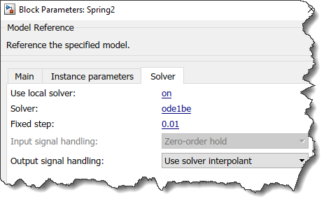
When referencing the model, in the dialog of the Model block, you will see a new "Solver" tab reporting which solver is being used:

To illustrate that, I put together a simple model referencing two other models, one simulating a stiff system solved with steps of 0.01 second using the ode1be solver, and the other a less stiff system solved using steps of 0.1 second using the ode1 solver. If I enable the logging of states in the top model and display the results in the Simulation Data Inspector with markers, I can see that they have been solved using a different step size:

Zero-Crossing Detection for Fixed-Step Solver
Another major addition to Simulink solvers is the possibility to detect zero-crossing events with fixed-step solvers.
In the Solver section of the model configuration, you will see this new option:

This setting can significantly improve the accuracy of models with fast switching dynamics that need to be solved using a fixed-step solver to enable deployment to hardware. The settings for maximum number of bracketing iterations and maximum number of zero-crossing per step can help ensuring that the generated code can respect real-time constraints.
Here is a simple model illustrating the impact of enabling fixed-step zero-crossing, notice how it improves the results compared to the variable-step reference:

If I run the model and compare the output of the Integrator block, we can clearly see the impact of fixed-step zero-crossing
mdl = 'testZC';
in(1:3) = Simulink.SimulationInput(mdl);
in(1) = in(1).setModelParameter('SolverType','Variable-step');
in(2) = in(2).setModelParameter('SolverType','Fixed-Step',...
'EnableFixedStepZeroCrossing','off');
in(3) = in(3).setModelParameter('SolverType','Fixed-Step',...
'EnableFixedStepZeroCrossing','on');
out = sim(in,'ShowProgress','off');
figure(1);clf
subplot(2,1,1)
plot(out(1).logsout.get("pulse").Values)
axis([0 10 -1.2 1.2])
subplot(2,1,2)
plot(out(1).logsout.get("integrator").Values); hold on;
plot(out(2).logsout.get("integrator").Values)
plot(out(3).logsout.get("integrator").Values,'-o')
legend({'Variable-Step','Fixed-Step No ZC','Fixed-Step ZC'},'Location','northwest')
Many Redesigned Apps
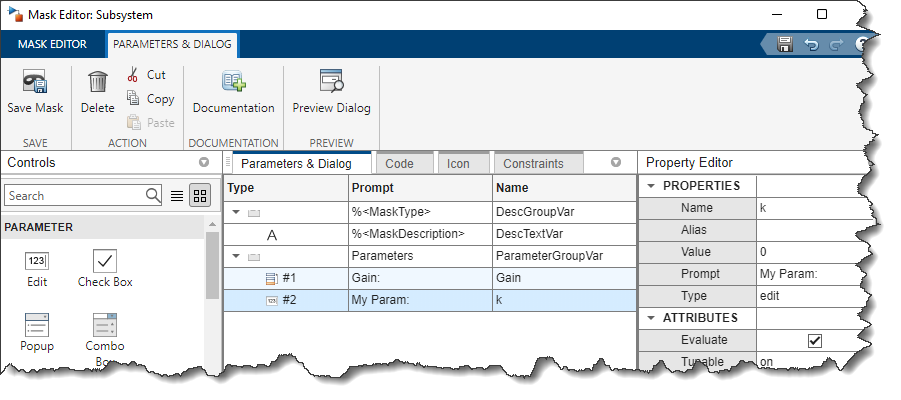
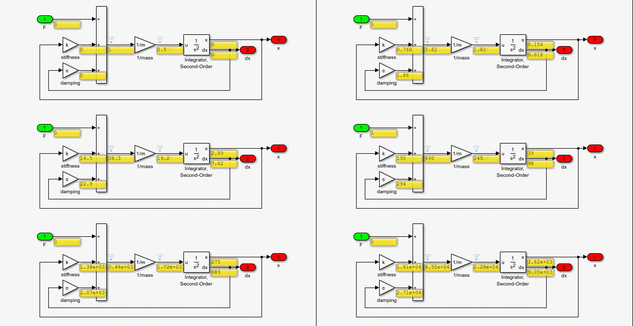
One last thing I want to point out about MATLAB R2022a is that multiple tools and apps have been redesigned for a more modern look and improved usability.
Here are a few examples:


Now it's your turn
Take a look at the R2022a release notes and let us know what your favorite feature is in the comments below.
If there is one feature in particular that you would like to see being covered in more details in this blog, also let us know in the comments.
- Category:
- What's new?


Comments
To leave a comment, please click here to sign in to your MathWorks Account or create a new one.