
Troubleshooting the Transport Delay Block
Yesterday I came across this model:

At first look, one might think that these two implementations should give the same results. However this is not the case because the delayed data is different.
I think this model is a good opportunity to explain a property of the Transport Delay block that seems to confuse many users.
The Question
When simulating the model, we notice that the output of the transfer function is different if the signal is delayed by two 2ms delays compared to one 4ms delay. The image below is a zoom on the transition at 4ms. We can see that the signal delayed by two 2ms delays start increasing before the simulation reaches 4ms.

The Investigation
In this model, the Transport Delay blocks have their initial conditions set to zero. Consequently, at 4ms the input signal to the Transfer Function jumps from 0 to 100.
The first thing I did was to look carefully at the input to the transfer function. If we zoom around the 4ms region, we can see that the signal delayed by two 2ms delays (blue) follows a slope between 3.8ms and 4ms. The signal delayed by one 4ms delay shows a perfect step at 4ms. (Note that I used the new feature I described last week to add markers on the Simulink Scope!)

You might want to notice that the duration of the ramp signal in this model is a function of the solver maximum step size. Changes to the solver settings will change the simulation results.
To find an explanation for this phenomenon, let's looks at the documentation:

In case you missed it, I highlighted an important requirement for the usage of this block: The input to this block should be a continuous signal. When we say continuous here, we do not only mean the the signal should have a continuous sample time, but also that the value of the signal changes smoothly (difference between two values should be small).
The explanation
As you can see in the documentation, the Transport Delay block interpolates linearly between points. This leads approximately to the following sequence of events:
- In this model, the maximum time step is 0.2ms
- At t=4ms, the transfer function blocks notice a large change in their output.
- The solver goes back in time to ~3.86ms, to ensure the tolerances are respected.
- At 3.86ms, the 4ms delay looks in its buffer. The desired value is before simulation start, so the transport delay outputs its initial condition.
- At 3.86ms, the second 2ms delay block look in its buffer. What it finds is one point equal to zero at t=1.8ms and one point equal to 100 at time 2ms. The second transport delay block interpolates between these 2 points and generates an output ~30
- The same process repeats for the other points interpolated between 3.8ms and 4ms.
Conclusion
The first 2ms delay in this model is generating a step at t=2ms. This step became the input to the second Transport Delay block. The step signal is not a continuous signal (continuous sample time and smoothly changing). This goes against the guidance specified in the documentation.
Of course, there are multiple ways to obtain the desired results. As it is often the case, the best solution will depend on the larger context into which this construct is used. For example, one way to avoid the step generated by the first 2ms delay is to set its initial value to 100. In that case the two 2ms delays will produce results identical to the 4ms delay.
Now it's your turn
Do you use the transport delay block? Did you ever got confused by this restriction on the signals you can feed to this block? Leave a comment here.
- Category:
- Modeling,
- Signals,
- Simulink Tips


Comments
To leave a comment, please click here to sign in to your MathWorks Account or create a new one.