
Deep Learning: Transfer Learning in 10 lines of MATLAB Code
Avi’s pick of the week is Deep Learning: Transfer Learning in 10 lines of MATLAB Code by the MathWorks Deep Learning Toolbox Team.
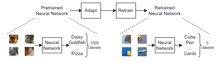
Have you ever wanted to try deep learning to solve a problem but didn’t go through with it because you didn’t have enough data or were not comfortable designing deep neural networks? Transfer learning is a very practical way to use deep learning by modifying an existing deep network (usually trained by an expert) to work with your data. This post contains a detailed explanation on how transfer learning works. Before you read through the rest of this post, I would highly recommend you watch this video by Joe Hicklin (pictured below) that illustrates what I will explain in more detail.

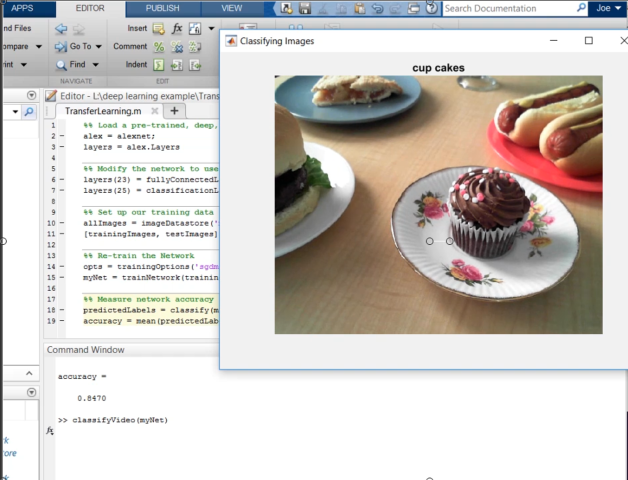
The problem I am trying to solve with transfer learning is to distinguish between 5 categories of food – cupcakes, burgers, apple pie, hot dogs and ice cream. To get started you need two things:
- Training images of the different types of food we are trying to recognize
- A pre-trained deep neural network that we can re-train for our data and task
Load Training Images
I have all my images stored in the “Training Data ” folder with sub-directories corresponding to the different classes. I chose this structure as it allows imageDataStore to use the folder names as labels for the image categories.

To bring the images into MATLAB I use imageDatastore. imageDataStore is used to manage large collections of images. With a single line of code I can bring all my training data into MATLAB, in my case I have a few thousand images but I would use the same code even if I had millions of images. Another advantage of using the imageDataStore is that it supports reading images from disk, network drives, databases and big-data file systems like Hadoop.
allImages = imageDatastore('TrainingData', 'IncludeSubfolders', true, 'LabelSource', 'foldernames');
I then split the training data into two sets one for training and the other for testing, the split I used is 80% for training and the rest for testing.
[trainingImages, testImages] = splitEachLabel(allImages, 0.8, 'randomize');
Load Pre-trained Network (AlexNet)
My next step is to load a pre-trained model, I’ll use AlexNet which is a deep convolutional neural network that has been trained to recognize 1000 categories of objects and was trained on millions of images. AlexNet has already learned how to perform the basic image pre-processing that is needed to distinguish between different categories of images in it’s early layers, my goal is to “transfer” that learning to my task of categorizing different kinds of food.
alex = alexnet;
Now lets take a look at the structure of the AlexNet convolutional neural network.
layers = alex.Layers
layers =

  25x1 Layer array with layers:

     1   'data'     Image Input                   227x227x3 images with 'zerocenter' normalization
     2   'conv1'    Convolution                   96 11x11x3 convolutions with stride [4  4] and padding [0  0]
     3   'relu1'    ReLU                          ReLU
     4   'norm1'    Cross Channel Normalization   cross channel normalization with 5 channels per element
     5   'pool1'    Max Pooling                   3x3 max pooling with stride [2  2] and padding [0  0]
     6   'conv2'    Convolution                   256 5x5x48 convolutions with stride [1  1] and padding [2  2]
     7   'relu2'    ReLU                          ReLU
     8   'norm2'    Cross Channel Normalization   cross channel normalization with 5 channels per element
     9   'pool2'    Max Pooling                   3x3 max pooling with stride [2  2] and padding [0  0]
    10   'conv3'    Convolution                   384 3x3x256 convolutions with stride [1  1] and padding [1  1]
    11   'relu3'    ReLU                          ReLU
    12   'conv4'    Convolution                   384 3x3x192 convolutions with stride [1  1] and padding [1  1]
    13   'relu4'    ReLU                          ReLU
    14   'conv5'    Convolution                   256 3x3x192 convolutions with stride [1  1] and padding [1  1]
    15   'relu5'    ReLU                          ReLU
    16   'pool5'    Max Pooling                   3x3 max pooling with stride [2  2] and padding [0  0]
    17   'fc6'      Fully Connected               4096 fully connected layer
    18   'relu6'    ReLU                          ReLU
    19   'drop6'    Dropout                       50% dropout
    20   'fc7'      Fully Connected               4096 fully connected layer
    21   'relu7'    ReLU                          ReLU
    22   'drop7'    Dropout                       50% dropout
    23   'fc8'      Fully Connected               1000 fully connected layer
    24   'prob'     Softmax                       softmax
    25   'output'   Classification Output         crossentropyex with 'tench', 'goldfish', and 998 other classes
Modify Pre-trained Network
AlexNet was trained to recognize 1000 classes, we need to modify it to recognize just 5 classes. To do this I’m going to modify a couple of layers. Notice how structure of the last few layers now differs from AlexNet
layers(23) = fullyConnectedLayer(5);
layers(25) = classificationLayer
layers =

  25x1 Layer array with layers:

     1   'data'    Image Input                   227x227x3 images with 'zerocenter' normalization
     2   'conv1'   Convolution                   96 11x11x3 convolutions with stride [4  4] and padding [0  0]
     3   'relu1'   ReLU                          ReLU
     4   'norm1'   Cross Channel Normalization   cross channel normalization with 5 channels per element
     5   'pool1'   Max Pooling                   3x3 max pooling with stride [2  2] and padding [0  0]
     6   'conv2'   Convolution                   256 5x5x48 convolutions with stride [1  1] and padding [2  2]
     7   'relu2'   ReLU                          ReLU
     8   'norm2'   Cross Channel Normalization   cross channel normalization with 5 channels per element
     9   'pool2'   Max Pooling                   3x3 max pooling with stride [2  2] and padding [0  0]
    10   'conv3'   Convolution                   384 3x3x256 convolutions with stride [1  1] and padding [1  1]
    11   'relu3'   ReLU                          ReLU
    12   'conv4'   Convolution                   384 3x3x192 convolutions with stride [1  1] and padding [1  1]
    13   'relu4'   ReLU                          ReLU
    14   'conv5'   Convolution                   256 3x3x192 convolutions with stride [1  1] and padding [1  1]
    15   'relu5'   ReLU                          ReLU
    16   'pool5'   Max Pooling                   3x3 max pooling with stride [2  2] and padding [0  0]
    17   'fc6'     Fully Connected               4096 fully connected layer
    18   'relu6'   ReLU                          ReLU
    19   'drop6'   Dropout                       50% dropout
    20   'fc7'     Fully Connected               4096 fully connected layer
    21   'relu7'   ReLU                          ReLU
    22   'drop7'   Dropout                       50% dropout
    23   ''        Fully Connected               5 fully connected layer
    24   'prob'    Softmax                       softmax
    25   ''        Classification Output         crossentropyex
Perform Transfer Learning
Now that I have modified the network structure it is time to learn the weights for the last few layers that we modified. For transfer learning we want to change the network ever so slightly. How much a network is changed during training is controlled by the learning rates. Here we do not modify the learning rates of the original layers, i.e. the ones before the last 3. The rates for these layers are already pretty small so they don’t need to be lowered further. You could even freeze the weights of these early layers by setting the rates to zero.
opts = trainingOptions('sgdm', 'InitialLearnRate', 0.001, 'MaxEpochs', 20, 'MiniBatchSize', 64);
One of the great things about imageDataStore it lets me specify a “custom” read function, in this case I am simply resizing the input images to 227×227 pixels which is what AlexNet expects. I can do this by specifying a function handle with code to read and pre-process the image.
trainingImages.ReadFcn = @readFunctionTrain;
Now let’s go ahead and train the network, this process usually takes about 5-20 minutes on a desktop GPU. This is a great time to grab a cup of coffee.
myNet = trainNetwork(trainingImages, layers, opts);
Training on single GPU.
Initializing image normalization.
|=========================================================================================|
|     Epoch    |   Iteration  | Time Elapsed |  Mini-batch  |  Mini-batch  | Base Learning|
|              |              |  (seconds)   |     Loss     |   Accuracy   |     Rate     |
|=========================================================================================|
|            1 |            1 |         2.32 |       1.9052 |       26.56% |       0.0010 |
|            1 |           50 |        42.65 |       0.7895 |       73.44% |       0.0010 |
|            2 |          100 |        83.74 |       0.5341 |       87.50% |       0.0010 |
|            3 |          150 |       124.51 |       0.3321 |       87.50% |       0.0010 |
|            4 |          200 |       165.79 |       0.3374 |       87.50% |       0.0010 |
|            5 |          250 |       208.79 |       0.2333 |       87.50% |       0.0010 |
|            5 |          300 |       250.70 |       0.1183 |       96.88% |       0.0010 |
|            6 |          350 |       291.97 |       0.1157 |       96.88% |       0.0010 |
|            7 |          400 |       333.00 |       0.1074 |       93.75% |       0.0010 |
|            8 |          450 |       374.26 |       0.0379 |       98.44% |       0.0010 |
|            9 |          500 |       415.51 |       0.0699 |       96.88% |       0.0010 |
|            9 |          550 |       456.80 |       0.1083 |       95.31% |       0.0010 |
|           10 |          600 |       497.80 |       0.1243 |       93.75% |       0.0010 |
|           11 |          650 |       538.83 |       0.0231 |      100.00% |       0.0010 |
|           12 |          700 |       580.26 |       0.0353 |       96.88% |       0.0010 |
|           13 |          750 |       621.47 |       0.0154 |      100.00% |       0.0010 |
|           13 |          800 |       662.39 |       0.0104 |      100.00% |       0.0010 |
|           14 |          850 |       703.69 |       0.0360 |       98.44% |       0.0010 |
|           15 |          900 |       744.72 |       0.0065 |      100.00% |       0.0010 |
|           16 |          950 |       785.74 |       0.0375 |       98.44% |       0.0010 |
|           17 |         1000 |       826.64 |       0.0102 |      100.00% |       0.0010 |
|           17 |         1050 |       867.78 |       0.0026 |      100.00% |       0.0010 |
|           18 |         1100 |       909.37 |       0.0019 |      100.00% |       0.0010 |
|           19 |         1150 |       951.01 |       0.0120 |      100.00% |       0.0010 |
|           20 |         1200 |       992.63 |       0.0009 |      100.00% |       0.0010 |
|           20 |         1240 |      1025.67 |       0.0015 |      100.00% |       0.0010 |
|=========================================================================================|
Test Network Performance
Now let’s the test the performance of our new “snack recognizer” on the test set. We’ll see that the algorithm has an accuracy of over 80%. You can improve this accuracy by adding more training data or tweaking some of the parameters for training.
testImages.ReadFcn = @readFunctionTrain;
predictedLabels = classify(myNet, testImages);
accuracy = mean(predictedLabels == testImages.Labels)
accuracy =

    0.8260
Try the classifier on live video
Now that we have a deep learning based snack recognizer, i’d encourage you to grab a snack and try it out yourself.
Also check out this video by Joe that shows how to perform image recognition on a live stream from a webcam.
- Category:
- Picks


Comments
To leave a comment, please click here to sign in to your MathWorks Account or create a new one.