Some time ago, I wrote a series of posts to highlight the different factors to take into account when trying to run simulations in parallel. In R2017a, we are making it significantly easier with the introduction of a new function: parsim

Let's see how that works!

Simulink.SimulationInput

If you are going to use the Parallel Computing Toolbox to simulate a model multiple times, there is obviously something you want to change to make each run different. This is done through the Simulink.SimulationInput object.

By creating one Simulink.SimulationInput per simulation, you can define the properties specific to each run, including initial states, model parameters, block parameters, input signals, and variables used by the model.

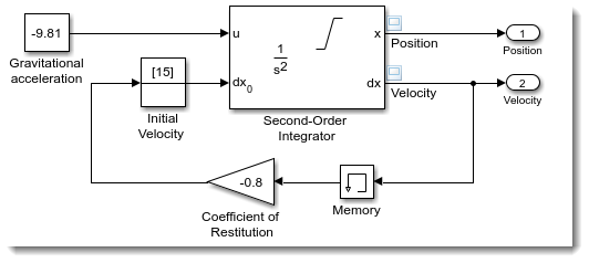
Let's take this simple bouncing ball model, and try to simulate it in parallel for different coefficient of restitution.

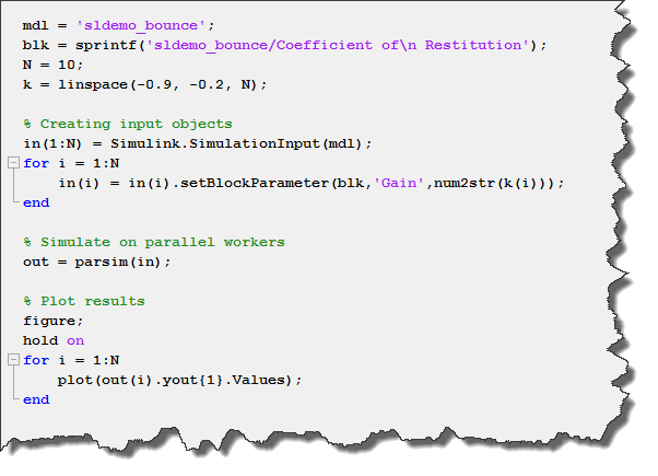
In this case, we will simulate the model for 10 different values, from 0.2 to 0.9. For that, I create an array of 10 Simulink.SimulationInput objects, and use the setBlockParameter method to specify the coefficient of restitution for each simulation. I can then simply pass this array of Simulink.SimulationInput to parsim, and I will receive as output an array of Simulink.SimulationOutput objects.

A More Realistic Example

Let's make this bouncing ball example more realistic by adding the following:

Workspace Variables: Before parsim, one of the challenges when simulating a model in parallel was to manage the variables needed by the model. I tried to provide tips and tricks to help with that in this previous post. For our bouncing ball example, instead of hard-coding the value of parameters like gravity and coefficient of restitution in block dialogs, let's have those be variables in the MATLAB base workspace, created by a MATLAB script.

Output Processing: In most cases, a simulation produces a large amount of data. If you are simulating on a remote cluster, you probably want to avoid transferring all this data. Instead, you can post-process the logged data and reduce it to what you are really interested in.

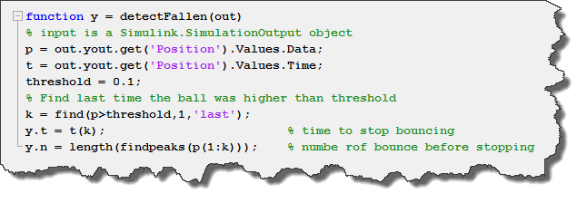
For the post processing, we need to create a function that receives as input the simulation output object and returns a structure output. For example, I can use the logged position to computer how long it took for the ball to stop bouncing, and how many rebounds it did.

With that setup, we can create our array of Simulink.SimulationInput object, and use the setVariable method to specify different values for the workspace variable Cr. For the post-processing function, we specify a handle to it to the postSimFcn property of the simulation input object.

Here is what it looks like:

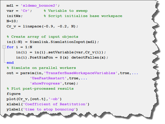
Notice how I also use the UseFastRestart option to speed things up even more by compiling the model only once on each worker.

Handling Errors

One of the thing I like about parsim is how it behaves when the simulation errors out.

In this case, the Simulink.SimulationOutput object contains all the logged data until the error happened, and a ErrorMessage field describing the cause of the error.

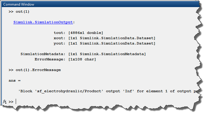
This is very useful to understand what went wrong without the need to re-simulate the model.

If you cannot figure out what went wrong based on the logged data, you will very likely want to add more instrumentation to the model and re-simulate it on your host machine. In that case, you will like the applyToModel method of the simulation input object. As its name implies,
this method will configure your current MATLAB session and model so that you can simulate it as it did on the worker.

Now it's your turn

Give a try at the new parsim function in R2017a and let us know what you think in the comments below.