Seth on Simulink

October 24th, 2008

Simulink models present a schematic layout of your algorithm.  The diagram encodes information about the system in the form of block icons, data type annotations, and sample time colors.  In technical support, I have seen many questions like,

• How can I print on a black and white printer and show sample time information?
• What is the sample time of the green signal?
• Why does Simulink have so few sample time colors?

In this post, I will to show you some new R2008b features that make it easier to understand what rates are in your model and make it easier to document your design.  I will also unravel the mystery of why Simulink has so few sample time colors.

Sample Time Annotations

For a long time Simulink has offered a Format menu option to turn on the sample time colors.  This labels blocks and signals with different colors based on their update rate.  Red for the fastest discrete rate, green for the second fastest, black for continuous, and many more.  The documentation has a table of sample time colors and their meaning.  After updating the diagram (Ctrl-D), these colors show you which blocks have the same rates in your model.  In Simulink R2008b, you can choose to show the sample time colors as well as sample time annotations.

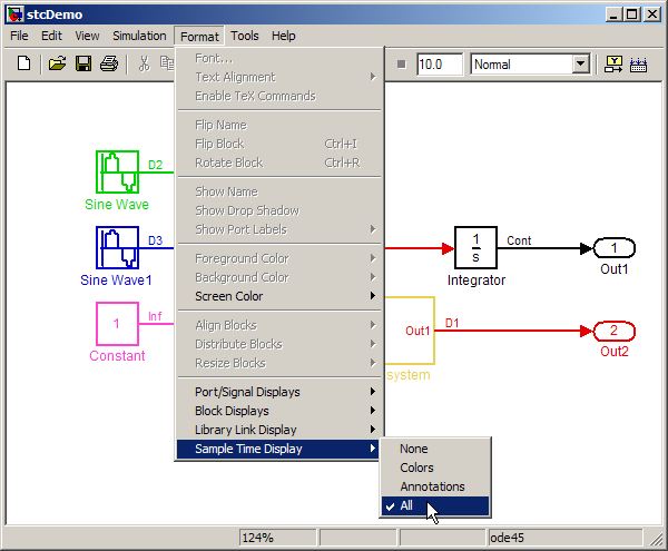
The annotations add text  to the diagram that identifies rates as D1, D2, D3, Cont, Inf, etc.  This is a great reminder when your model has many rates in it.  Now you can print your model on a black and white printer and keep the rate information visible in the form of annotations.

The Sample Time Legend

To help decode the meaning of these annotations and the colors, we have added the Sample Time Legend.  This opens when you first enable the Sample Time Display options, and is also found through the View->Sample Time Legend menu.

The annotation labels show you the meaning of the color and include the value of the sample time for that model.  In previous releases, you could only get a list of sample times in the model using debugger commands.  For example:

Why so few sample time colors?

Simulink graphics originally (circa 1992) had a minimum 16-color graphics environment, including X terminals and Windows 3.0. This meant that the lowest common denominator had to work. All the color stuff was hard-coded into the sample time code, so even when 32-bit core color support was added circa R12-R13, the sample time code was not updated. The addition of annotations and a sample time legend are part of a much larger project in recent releases to improve the use of color in Simulink.

Do you have sample time colors turned on in your models?  Leave a comment and tell me what you think about this new feature.

10:30 UTC | Posted in History, Simulink Tips, What's new? | Permalink |

You can follow any responses to this entry through the RSS 2.0 feed. You can skip to the end and leave a response. Pinging is currently not allowed.

6 Responses to “R2008b Simulink: Sample Time Colors”

1. Han Geerligs replied on October 29th, 2008 at 02:52 UTC :
   

   Hi Seth,

   as an enhancement maybe you could add the value of the sampletime to the annotation e.g. D1 [0.01 0] which means: discrete sampletime 1 with Tsample=0.01 and offset=0;

   Btw: I was wondering in which situations the offset is chosen unequal to zero: in my daily work I never encounter such a situation?

2. Arwen Warlock replied on October 29th, 2008 at 12:50 UTC :
   

   Regarding adding the sample time to the annotation, we considered this, and even prototyped it. We found that it made the diagram really busy for two main reasons: 1) the sample times frequently require 5 or more significant digits to represent, and 2) the sample time annotations have to share screen real estate with the data types, dimensions, signal names, and other properties that can be displayed on the lines.

3. Seth replied on October 29th, 2008 at 21:30 UTC :
   

   For those of you who don’t know Arwen, she is the developer who added the sample time annotations and the sample time legend.

   @Arwen - Thanks for providing some background on the feature you have been working so hard on.

   @Han Geerligs - The offset can be used to distribute the execution of slow tasks across multiple fast task steps. Consider an embedded system that runs a 10 ms base task, and 4 systems that need to be updated at 40 ms. These 4 can be scheduled with offsets so that only one runs at each 10 ms task, thus not overwhelming the processor, and not requiring premptive multitasking.

   [10 0] tid 1 (base task)
   [40 0] tid 2 (slow task 1)
   [40 10] tid 3 (slow task 2)
   [40 20] tid 4 (slow task 3)
   [40 30] tid 5 (slow task 4)

4. Han Geerligs replied on October 30th, 2008 at 07:09 UTC :
   

   @Arwen: thanks for the explanation, it was also my (wild) guess that this would be the reason.
   How about printing the legend along with the model?

   @Seth: thanks for the explanation as well!

5. Arwen Warlock replied on October 30th, 2008 at 08:31 UTC :
   

   @Hans: Thanks for the question. Unfortunately, printing the sample time legend is not available in R2008b. Watch the announcements from the MathWorks for future releases.

6. Jim replied on November 11th, 2008 at 14:11 UTC :
   

   Note that you can still print the sample times using the sim command:

   sim(bdroot,[],simset(’Debug’,{’stimes’,’stop’}))

   This can be included as text in a report via Report Generator.

Leave a Reply

<pre class="code">
a = magic(3);
sum(a)
</pre>

These postings are the author's and don't necessarily represent the opinions of The MathWorks.