Guy and Seth on Simulink

January 30th, 2009

MathWorks Conversations and the FFT

If you are like me, you read the doc, a lot. I am often clicking on the help just to verify my understanding of a function’s syntax, or the behavior of a block. That is why I wasn’t surprised to find myself involved in a detailed discussion about the documentation for FFT.

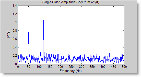
You go it… just another day at the MathWorks. For some context, the doc example generates a signal corrupted with noise, and then uses the FFT to extract the frequency components.

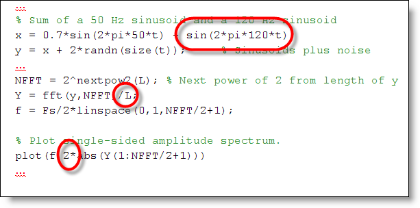
Fs = 1000;                    % Sampling frequency
T = 1/Fs;                     % Sample time
L = 1000;                     % Length of signal
t = (0:L-1)*T;                % Time vector
% Sum of a 50 Hz sinusoid and a 120 Hz sinusoid
x = 0.7*sin(2*pi*50*t) + sin(2*pi*120*t);
y = x + 2*randn(size(t));     % Sinusoids plus noise
plot(Fs*t(1:50),y(1:50))
title('Signal Corrupted with Zero-Mean Random Noise')
xlabel('time (milliseconds)')

Noise corrupted signal plot

NFFT = 2^nextpow2(L); % Next power of 2 from length of y
Y = fft(y,NFFT)/L;
f = Fs/2*linspace(0,1,NFFT/2+1);

% Plot single-sided amplitude spectrum.
plot(f,2*abs(Y(1:NFFT/2+1)))
title('Single-Sided Amplitude Spectrum of y(t)')
xlabel('Frequency (Hz)')
ylabel('|Y(f)|')

FFT spectrum plot

There were two questions that started the discussion. The first one,

Why does the FFT example in the doc have so much code?

We can ignore that for now and focus on the second question, and the real meat of the discussion:

Why does the FFT example result in an amplitude of 1?

My colleague Jeoffrey surprised me with his intimate familiarity with the discrete time Fourier transform and his ability to produce the complicated equations out of thin air. I told him, “I want that in a blog post!” So here it is. Today’s featured guest blogger is Jeoffrey Young:

Jeoffrey Young, FT and DTFT Expert

Why does the FFT example result in an amplitude of 1?
By Jeoffrey Young

In this post I will talk about one way of looking at where the scaling comes from in the following example from Matlab 7.7 (R2008b)’s help documentation:

MATLAB code for the FFT circled

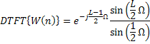
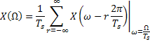
To start with, let’s remember that FFT is simply the sampled Discrete Time Fourier Transform of a signal. We know from DTFT that (I’ll use the cosine function here for simplicity):

where and (Ever wonder why this looks exactly the same as the Fourier Transform of the continuous time cosine signal? More on this later.) However, it is not enough to sample a continuous time signal that is not time-limited, such as a cosine function. Truncating so that we can represent the signal on a computer is equivalent to multiplying the time-domain signal by the following rectangular window:

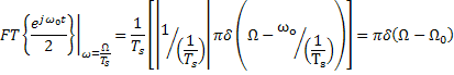
The DTFT of this signal is the Digital Sinc Function:

Note that by L’Hopital’s Rule.

Thus, from the time-domain multiplication property of Fourier Transform:

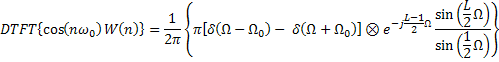
Here we see that the DTFT of an L-point truncated cosine function has a maximum amplitude of (if we ignore the effects of aliasing from the overlap and the fact that DTFT is periodic).

Question about the scale factor used with FFT are also sent to technical support. This happens often enough that tech support posted a solution titled “Why is the example of using an FFT to get a frequency spectrum scaled the way it is?” We even have a technical note on the general topic of spectral analysis with FFT: Tech Note: 1702 - Using FFT to Obtain Simple Spectral Analysis Plots. As we see it used in this post, the section below describes how the scale factor may also depend on the signal of interest.

Why does looks exactly like ?

Remember the following relationship between the DTFT of the sampled analog signal and the FT of the original signal:

In other words, the Discrete Time Fourier transform is scaled by . However, the DTFT of a sinusoid is the Delta Function, which is defined more by its properties than its value. Thus, its amplitude has to be scaled when the axis is modified :

So that:

Now it's your turn

If you have any thoughts on how scaling the FFT results may be useful, please post your comments here.

By Seth Popinchalk

12:27 UTC | Posted in Fundamentals, Guest Blogger, Signal Processing | Permalink | 10 Comments »

You can follow any responses to this entry through the RSS 2.0 feed. You can skip to the end and leave a response. Pinging is currently not allowed.

10 Responses to “MathWorks Conversations and the FFT”

Saurabh replied on February 28th, 2009 at 09:35 UTC :

Sir,
I have tried a lot but i am unable to find fft in simulunk. Can you tell me which block should i use to find fft and which scope block to see it?
Thankyou.
Seth replied on March 1st, 2009 at 21:58 UTC :

@Saurabh – The blocks I think you are looking for are part of the Signal Processing Blockset. You can find an FFT block in the Power Spectrum Estimation library. There is also a Spectrum Scope in the Signal Processing sinks. If you don’t have the Signal Processing Blockset, output your signal data to the MATLAB work space and compute and FFT from there. I hope that helps.
Prashant replied on November 12th, 2009 at 15:47 UTC :

How can I have same example but instead AC(1 to 10V 50 or 60Hz) and DC(0.5 to 10 V) then adding AC+DC but out put should be only DC signal? I will be very glad to know if this kind of*. m code can be transferred to simulink block where the block accepts AC+DC as input and the out put as DC signal only.

This example is quite good to know.
Jay replied on May 25th, 2010 at 16:42 UTC :

Thanks for this. It answers most of my questions. Can you recommend a good, IN PRINT reference text that covers all of these issues? Another one that isn’t well covered is how to convert DFT’s between “normalized” and un-normalized frequencies. The reference texts you give are all dated and mostly out of print; or they cover one issue but not the others.

Thanks again.
Jeoffrey replied on May 30th, 2010 at 21:40 UTC :

@Jay – I’m glad this helped! Any Digital Signal Processing text should cover this material. For example, the text “Discrete-Time Signal Processing by Oppenheim, A. V. and R. W. Schafer” should still be in print. As for the different time a frequency terminologies used in MATLAB, the following help documentation provides the complete list:

http://www.mathworks.com/access/helpdesk/help/toolbox/dspblks/ug/f13-54010.html#f13-23126
Dragan replied on June 10th, 2010 at 17:42 UTC :

Dear Seth,
I’m starting with just a frequency response and I’m having trouble re-adjusting the response( ie scaling) such that ifft could be used to generate a time domaine response. Here is a sample code that I’ve generated for a one simple transfer function example(ie g(jw)=1/(jw+1)).
```
k=1;
p=-1;
dt=1e-2;
tstop=30.01;

%Time period
t=0:dt:tstop;

%Apply  Freq Response
freq=0:1/tstop:1/dt;
jw=j*2*pi*freq;
w=2*pi*freq;
for d=1:length(freq)
    g(d)=k/(jw(d)-p);
end
% %double sided response
n=length(g)
m=fliplr(conj(g(2:((n)/2+1))));
mm=[g(1:(n)/2) m]*n;
 x=real(ifft(mm))/tstop;
plot(t,x)
hold on
 %Known Time domain result from Laplace
 for d=1:length(t)
   h(d)=exp(p*t(d));
 end
plot(t,h,'r')
```
How would I handle the maximum frequency point with an even number of points? Is my scaling of my result correct? I hope that you can help me clear the issues behind ifft/fft. Thanks once again,

Dragan
Chai replied on July 23rd, 2010 at 22:51 UTC :

Hi Seth,
I am having a scaling problem with performing FFT in Simulink as well. When the output is displayed on a vector scope the resulting magnitude is too high compared to the theoretical value. While this alone is not the problem. The amplitude varies with FFT length and with the stop time too.
Any suggestions on scaling it appropriately?

Regards,
Chai
Issopui replied on July 25th, 2010 at 21:23 UTC :

Hi Seth,

Thanks for the naswer regarding Saurabh’s question. I’am having the same problem. I don’t have the Signal Processing Blockset install in my Matlab. I wanted to write a script to generate it form my output signal. As a newbie with Matlab I don’t really know how to introce the time and the different part of the script. This is what I have writen but it doesn’t work.
dt = 1/100;
T = 100;
t = (0:dt:T-dt);

x1 = voltage2.signals.values(:,1);
y = fft(x1)/length(x1)*2;
m = abs(y);
m(1)= m(1)/2;
f = (0:length(y)-1)*100/length(y);
plot(f,20*log10(m)),

hold on
ylabel(‘Abs. Magnitude dB’),

x2 = voltage3.signals.values(:,1);
y = fft(x2)/length(x2)*2;
m = abs(y);
m(1)= m(1)/2;
f = (0:length(y)-1)*100/length(y);
plot(f,20*log10(m),’-.’),
axis ([0 max(f)/2 -60 10])
hold off
h = legend(‘Uu’,'Uu0′);

It’s the ouput voltage of a 2 level 4 quadrant IGBT circuit.
X1 is the line to virtual neutral of the “Y” connected out put load voltage and X2 is the line to ground load voltage.
Please could u help me.
Many thanks.
Amit replied on December 21st, 2011 at 16:44 UTC :

Hello,

I think it would be useful to have a matlab function that directly computes time domain response from s-domain system transfer function available only as numerical data:
G(s=jw). While I realize there are subtleties in the FFT and iFFT scaling I’d rather not be bothered by these issues, since my focus is on dyanmics rather than signal procressing techniques and algorithms.

Amit.
Xianyu replied on January 7th, 2012 at 19:51 UTC :

Dear Sir,

I have a problem at hand that requires urgent attention. Thing is I’ve never used Simulink before and right now its required for me to FFT a continuous signal output from my vehicle model.

Thing is it is a continuous signal and I am facing problems trying to even implement the FFT. Even when there is no errors there would not be any output. So yes i’m desperate for help.

thanks.
XY