This week Matt Brauer is back to describe work he did to analyze the trajectory of the Hyperloop proposal. This is a key input to the Hyperloop Simulink models we are building.

Matt's conclusion is surprising:
From the perspective of geographic constraints and rider comfort, the 760 mph peak speed is not an issue. It’s the 300 mph section through the suburbs of San Francisco that requires closer consideration.

Where is the Hyperloop going?

As mentioned in a previous blog post, we’ve begun implementing Simulink models of the Hyperloop concept. To exercise those models, a core piece of information is the trajectory. We need to know where the Hyperloop is going and at what speed. I analyzed the proposal to derive this information, and what I found was interesting. From the perspective of geographic constraints and rider comfort, the 760 mph peak speed is not an issue. It’s the 300 mph section through the suburbs of San Francisco that requires closer consideration.

Potential Hyperloop route, including image from and Google Earth

The basic idea put forth in the proposal is to follow existing highways as much as possible. In order to limit lateral accelerations experienced by the passengers to 0.5g, there needs to be “minor deviations when the highway makes a sharp turn”. I remember from Freshmen Physics class that centripetal acceleration in a curve is proportional to the square of velocity. This means that increasing your velocity from 76 to 760 mph is actually a 100x multiplication of g forces.

Is it really possible to average 600 mph across the state of California on available land without making passengers nauseous? Or would a reasonable trajectory require wide loops, impeding on private citizens’ backyards? I put the technical computing power of MATLAB to work on answering these questions.

Technical Computing of a Route

I won’t go into all the details because this is a Simulink blog, but here is an overview of the steps I followed:

• First, I used Google Earth to get a set of longitude and latitude points along the California highways I-5 and I-580. After getting directions, saved a KML file with the data.
• I used the read_kml submission from the MATLAB Central File Exchange to import the data in MATLAB.
• It is possible to use functions like wmsfind, wmsupdate and wmsread from the Mapping Toolbox to add topography data to the route and surrounding area. However, I only used this information for plotting. For this first study, the derived route is only 2-dimensional.
• This gave me a set of discrete points along the highways, to which I associated a desired velocity based on the Hyperloop document.
• From these target points, I created a smoothed trajectory using the fit function from the Curve Fitting Toolbox.
• Using this smoothed trajectory, I wrote a simple script to calculate and plot the lateral acceleration along this trajectory.
• For the portions of the trajectory that were exceeding 0.5g's, I adjusted some target points to drive lateral accelerations below 0.5g’s while staying as close as possible to the original route.

In the end, I got the results below:

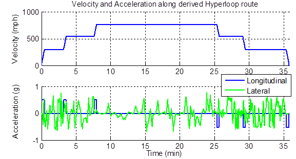
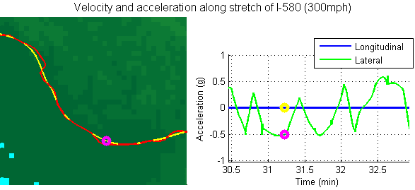
Velocity and Acceleration along derived Hyperloop route (created using the Mapping Toolbox)

You can see that the travel time is very close to the advertised 35 minutes. The accelerations were kept within reason, although it looks like a pretty dynamic ride.

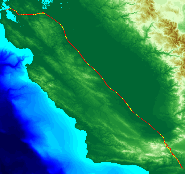
How much does the Hyperloop need to deviate from the existing highways in order to achieve these results?

The red line shows the targeted highways. The yellow portions show sections of the derived Hyperloop route that deviate from the mean highway route by more than 50m. The yellow, "off-highway", portions account for 113 miles of the 347 mile trip.

To review in depth, I wrote the trajectory back to KML using kmlwriteline from the Mapping Toolbox. Now it's possible to view the derived route in Google Earth.

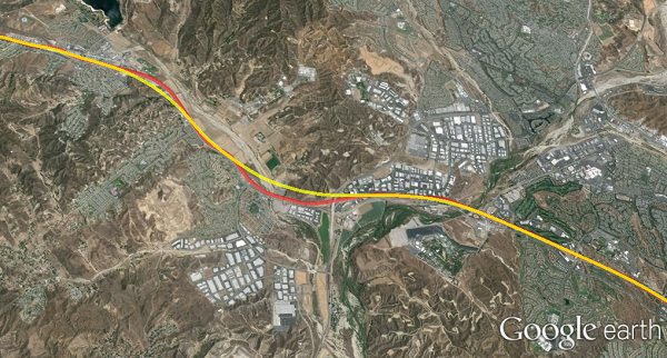
No major issues seen along I-5 (Image created using Google Earth)

Again, the red line is the mean highway route. Here, the yellow line shows the complete derived Hyperloop route. Upon reviewing the details, the route seems pretty reasonable up until I-580 outside of the bay area.

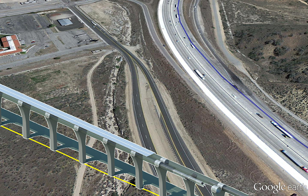
When I-580 turns west and starts going through the San Francisco suburbs, it becomes difficult to stay on the road. Here’s a snapshot of a particularly rough curve:

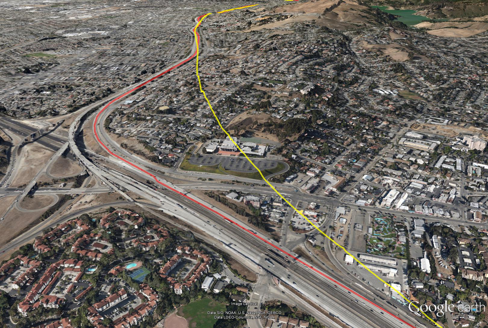
Re-routing along I-580 to avoid excessive g-forces (Image created using Google Earth)

Below is the route data for the area surrounding the above curve.

Despite the issues highlighted above, the final conclusion is quite positive. It seems that the first 295 miles of the route can be accomplished in about 27 minutes without excessive g’s on the passengers or encroaching on private property. “Landing” in the Bay Area may take a bit longer than originally advertised, but that seems like splitting hairs at this point. Further investigation is certainly warranted. So, let’s get those Simulink models running!

Now it's your turn

What do you think? Is the Hyperloop going in the right direction?

Given Elon Musk's statement that the Hyperloop should be an open design concept, would you be interested use Matt's trajectory and begin filling some of the boxes in our Hyperloop model architectures?

Let us know what you think by leaving a comment here.