Introducing the System Toolboxes
This week I am teaming up with my colleague Ken Karnofsky to introduce another big change in MATLAB R2011a.
Guy: So Ken, what is this big change?
Ken: In MATLAB R2011a, not only the code generation products changed. The products for designing signal processing algorithms have also been reorganized. Here is a visual summary what’s happening:

Guy: What is a System Toolbox?
Ken: Last year, we introduced a new technology in several blocksets called System objects. System objects are pre-defined algorithms for MATLAB with functionality that had previously been available only to Simulink users, such as fast stream processing, implicit state handling, design options such as fixed-point, and code generation support.
With the System Toolboxes, you can design signal processing algorithms suitable for fast simulation, real-time prototyping, and embedded implementation. Any MATLAB algorithm that you design for code generation, including the use of System objects, is reusable in Simulink using the new MATLAB function block.
Guy: That sounds pretty cool. Let's see how we can identify a system using an LMS adaptive filter, and implement it in 3 different ways:
MATLAB script
In this example, I create a dsp.LMSFilter object and a dsp.DigitalFilter object. Then I use the step method to process data using the algorithm defined by each objects. Executing step 10 times in a loop is similar to running a Simulink model for 10 time steps.
% Create adaptive filter object
hlms = dsp.LMSFilter(11, 'StepSize', 0.01);
% Create system to be identified... an FIR filter.
hfilt = dsp.DigitalFilter('TransferFunction', 'FIR (all zeros)', ...
    'Numerator', fir1(10, .25));

% Run 10 iterations of filter adaptation
for i = 1:10
    % Input to the system
    x = randn(100,1);
    % We measure some output to the system, including noise
    d = step(hfilt, x) + 0.01*randn(100,1);
    % Now let's run our adaptive filter
    [y,~,w] = step(hlms, x, d);
    % compare the measured and identified outputs
    diff(i) = sqrt(sum((y-d).^2));
end
After writing this script, I can see advantages of using System objects. After I initialize the object, all I have to do is call the step method in a loop to process data. The implementation of the step method is very efficient because it does not include the same overhead normally required for MATLAB functional programming.
If your goal is to target an embedded processor, you can use MATLAB Coder and generate C code directly from this algorithm. If you want to integrate this algorithm into a Simulink model...
MATLAB Function Block
With the MATLAB Function block and System objects, it is easy to bring an algorithm created in MATLAB into Simulink. To implement the same adaptive filter example, I made the following model:

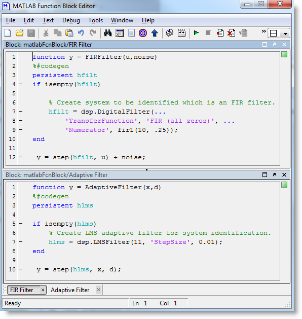
Then I define the FIR Filter and Adaptive Filter in the MATLAB Function block. I initialize the System objects on the first time step of the model and declare them as persistent so they can keep their states between each time step.

Of course it is possible to combine many System objects inside one MATLAB Function block and create more complex components.
Simulink blocks
For users who prefer just connecting blocks without typing code, don't worry! The System Toolboxes include ready to use Simulink libraries. The blocks in the Simulink libraries use the same System objects under the hood. For this example, here is how my model looks implemented using blocks from the DSP System Toolbox:

Now it’s your turn
Are you going to try the new System objects in your MATLAB code? Are you using MATLAB algorithms in your Simulink models? Let us know by leaving a comment here.


댓글
댓글을 남기려면 링크 를 클릭하여 MathWorks 계정에 로그인하거나 계정을 새로 만드십시오.