In honor of the first anniversary of Elon Musk's announcement, this week, Matt Brauer takes a look back at the evolution of our discussions on the Hyperloop transportation concept. To keep it interesting, we’re offering a dynamic vision of a Hyperloop trip from Southern California to the Bay Area.

A Look into the Future?

We’ve been publically developing a Simulink model of the Hyperloop for some time now. We recently looked into using MATLAB interfaces to visualize that journey in GoogleEarth. To create a virtual cockpit, we constructed a MATLAB figure combining GoogleEarth windows and several other native graphics capabilities. We think the resulting video is pretty cool.

http://youtu.be/n1csKKXuBrU

To understand how we arrived at this vision of the future, here’s a look back at our past Hyperloop posts.

Getting Started

We started out with a conversational post about Elon Musk’s concept and outlining some of the interesting technical points. This post was criticized for not brining any value to the discussion. I guess we were simulating trolling.

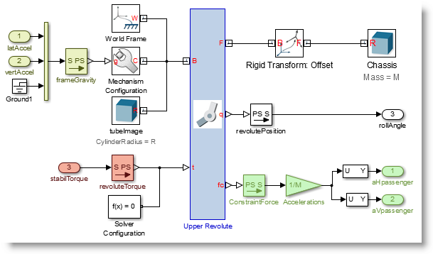
To get things moving, we introduced different approaches to architecting a simulation model for such a system. Guy suggested splitting the model into a plant (physical elements) and a controller (functional software) as in conventional model-based design. I proposed a more distributed architecture with several functional components, each containing its own plant and controller (image below). Guy’s proposal included subsystem variants while mine leveraged model reference.

click to enlarge

Initial dynamic analysis

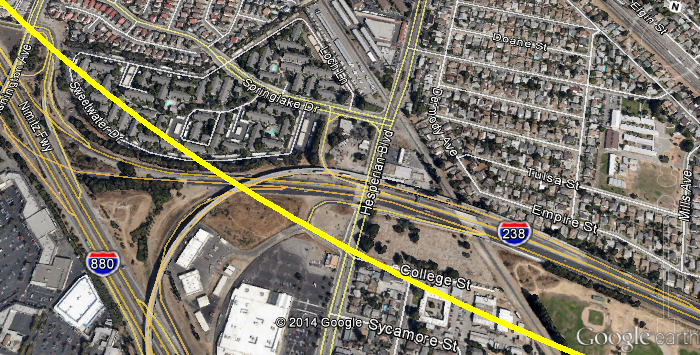
Last November, we published a two-dimensional analysis of the Hyperloop’s proposed route. We used the original proposal’s design constraints for curve radius to see how the track could be laid out over the California terrain.

The results highlighted the difficulties in maintaining tolerable g-levels for passengers while traveling at such high speeds along existing infrastructure. However, the analysis did not include several important factors; elevation and banking. Elevation promised to make route planning more difficult, while the effects of banking the vehicle in the tube would help reduce the g-forces and potentially improve the route.

Anticipated hyperloop route (yellow) to avoid excessive g-forces (Image created using Google Earth)

Promoting Collaboration

For Valentine’s Day, we used Simulink Projects to package a Simulink model on the MATLAB File Exchange that contained elements of each of our architectural approaches. My partitioning remained but now utilized Guy’s idea of using subsystem variants.

In April, R2014a was released with Simulink Projects supporting Git as a version control system. So, we quickly jumped on the bandwagon and placed an updated Hyperloop model on GitHub.

Improved dynamics

In May, we investigated the elevation profile of the route. We used optimization techniques to find the best combination of pillars and tunnels to meet cost and comfort demands. There were some great improvement suggestions in the comments of this post that we’ve yet to implement.

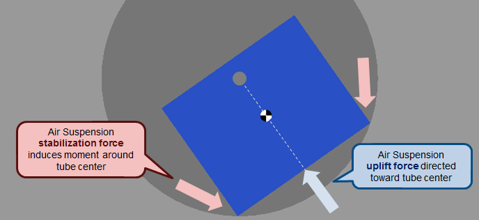
Last month, we enhanced the model to include the effects of banking within the tube. We blogged about a simple approach in SimMechanics to model those dynamics.

Roll your own!

In keeping with our collaborative mindset, the necessary models and m-scripts to generate this video are now available on the GitHub submission.

The project has even been set up to support new routes. Load your own KML file and see how the Hyperloop looks in your neighborhood.