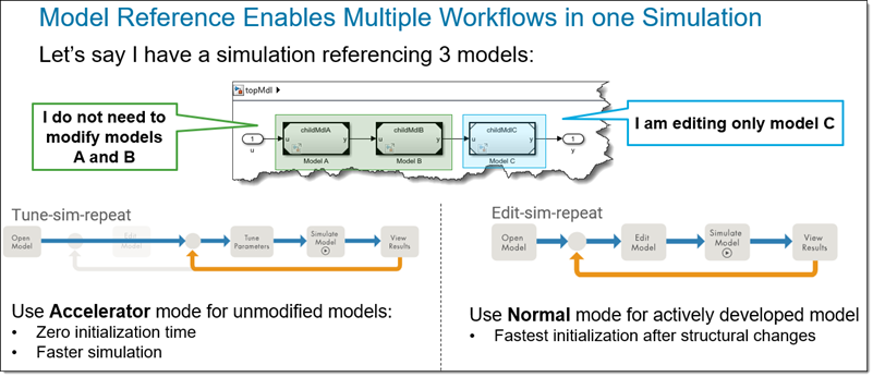
I recently attended the MathWorks Automotive Conference. This was a great opportunity to connect with industry experts and see how they use MATLAB and Simulink.During the conference, I gave a... read more >>

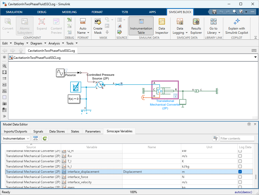
Did you know that starting in R2024a, it is possible to log Simscape variables like if they were Simulink signals?Let's see how that works.The ProblemHere is a pattern I often see in Simscape models.... read more >>

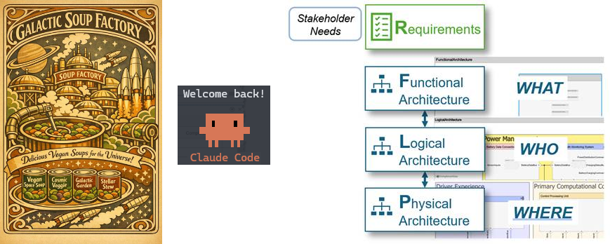
Today I am happy to welcome Sarah Dagen from MathWorks Consulting Services to talk about her experience with coding agents for Model-Based Systems Engineering..Like many of you, I’ve been exploring... read more >>

MATLAB R2026a is available, let's see what's new in the Simulink world.New Context MenuThis one cannot be missed! We decided to modernize our right-click menu.Here is what it looks like when you... read more >>

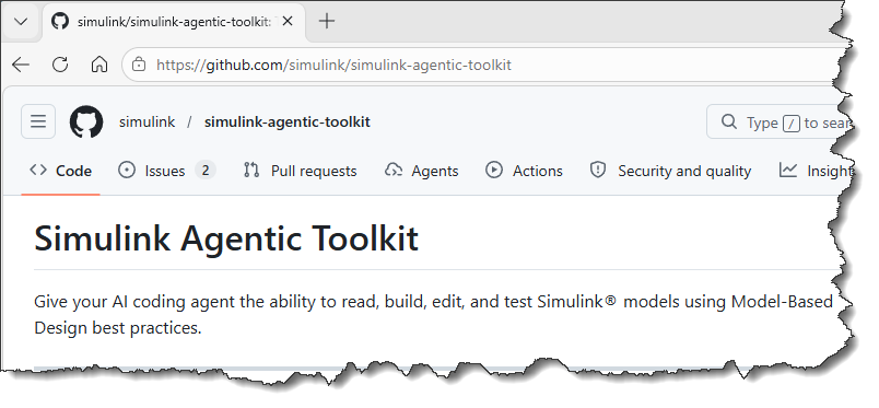
After the MATLAB Agentic Toolkit debuted last week, we are very happy to release the Simulink Agentic Toolkit on GitHub today.SetupTo get started, go through the README.md. You will see that it's as... read more >>

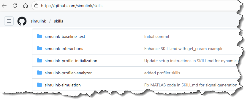
Update: The Simulink Agentic Toolkit is now available. I recommend installing the toolkit when interacting twith Simulink through an AI agent. Skills in this repository are complementary and should... read more >>

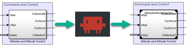
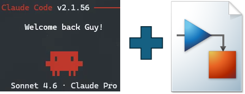
Once you start using those AI agents, it's hard to stop!In today's post, I used Amp, an AI coding agent made by Sourcegraph and similar to Claude Code, to do one of the tasks I help Simulink users... read more >>

This week, I am going one step further in my exploration of AI agents and how they can help Simulink workflows. In previous posts, I went through the basics of connecting GitHub Copilot with the... read more >>

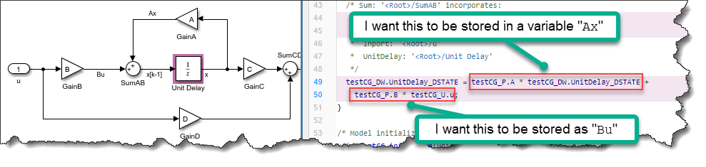
One of the key benefits of Simulink is that you can generate C/C++ code from the model using Simulink Coder and Embedded Coder.However, I have to admit, looking at the code generated from Simulink... read more >>

In my previous post, I went through the basics of using GitHub Copilot and the MATLAB MCP Server to generate MATLAB code that can simulate a Simulink. While the AI-generated code simulated the... read more >>