Guy and Seth on Simulink

December 24th, 2009

Today I introduce guest blogger Arkadiy Turevskiy to share some new features in R2009b: the PID Controller Blocks in Simulink and a new PID tuning method in Simulink Control Design.

PID (Proportional-Integral-Derivative) control seems easy: you just need to find three numbers: proportional, integral, and derivative gains. Many PID tuning rules exist out there and all you need to do is pick up one and press a button on a calculator. Easy enough, right? Unfortunately, the story is more complicated than that. Popular PID tuning methods are restrictive. For example, to use one of the most popular methods - Ziegler-Nichols - you need a stable, first order plus dead-time linear time-invariant (LTI) plant model. Even if your model is of that type, the method does not support tuning of integral or proportional-derivative controllers, and for the types of PID controllers it supports, it only provides one answer with no easy way to fine-tune the design. Moreover, tuning is not the only challenge. Real-life PID implementation also needs to consider such issues as output saturation, integrator wind-up, and discrete-time implementation.

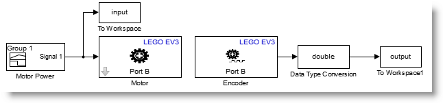
In R2009b we released new blocks in Simulink and a new PID tuning method in Simulink Control Design that together address these challenges. To see how this works, let’s consider an example of designing a PID controller for a dc motor. The model of a closed loop system uses the new PID Controller block. This block generates a voltage signal driving the dc motor to track desired shaft rotation speed. In addition to voltage, the dc motor subsystem takes torque disturbance as an input, allowing us to simulate how well the controller rejects disturbances. We also modeled analog sensor noise in the speed measurement.

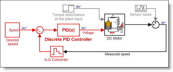
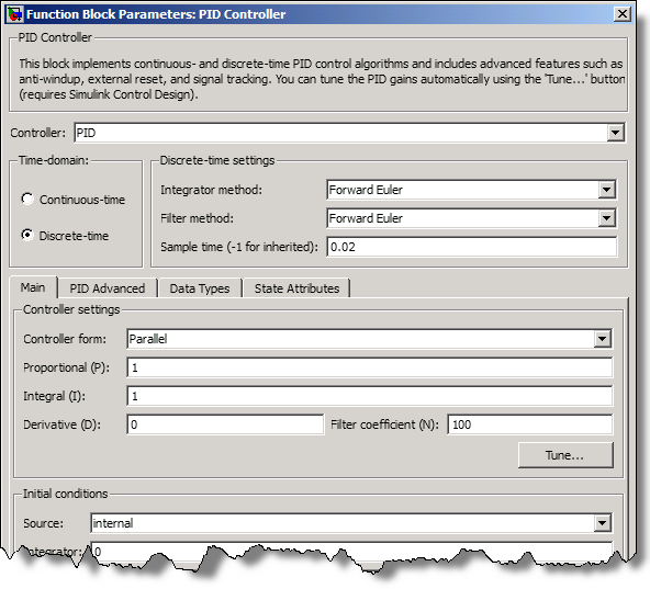
The PID controller is a discrete-time controller running at 0.02 seconds (the red color shows the sampling time in the model). Let’s now look at the dialog of the PID Controller block. In the upper half of the dialog we specified basic configuration of the PID controller: type (PID, PI, PD, P, or I), time-domain, integration methods, and sample time. In the lower part, we specified PID controller form and gains (shown at default values).  Block documentation provides detailed information about the block and all its parameters.

PID Tuning

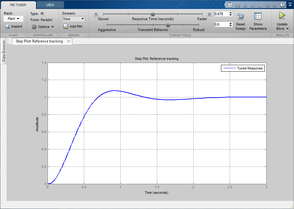
Our first task is to tune the PID controller. Pressing the “Tune…” button in the PID Controller block dialog, we launch PID Tuner, which linearizes the model at the default operating point and automatically determines PID controller gains to achieve reasonable performance and robustness based on linearized plant model.

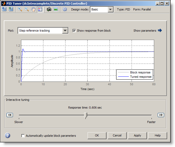
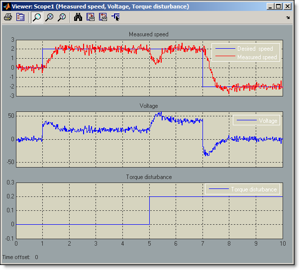
The grey line shows the system step response for the gain values currently defined in the block dialog, and the blue line shows the system response for the gain values that PID Tuner proposes. We can simply accept the proposed design and then run our closed-loop Simulink model to check the results. In the simulation, we command a step change from 0 to 2 rpm at 1 second and a step down to -2 rpm at 7 seconds. Results demonstrate good tracking with zero steady-state error, fast rise time, low overshoot, and good torque disturbance rejection (torque disturbance is modeled as a step change from 0 to 0.2 Newton-meters at 5 seconds). The tuning algorithm we just used works on any type of plant model, tunes all forms of PID controllers that can be specified in the PID Controller block, and takes sampling effects into account during the tuning process.

If system response does not meet our requirements, we could further fine-tune the design by interactively making the controller faster or slower, using the slider on the bottom of the PID Tuner GUI.

Integrator Anti-Windup Protection

We now run a different scenario, assuming no torque disturbance and assuming that the amplitude of voltage fed to the dc motor cannot exceed 10 Volts – to protect the motor from overheating. We use the “PID Advanced” tab of the PID Controller block dialog to specify these saturation limits.

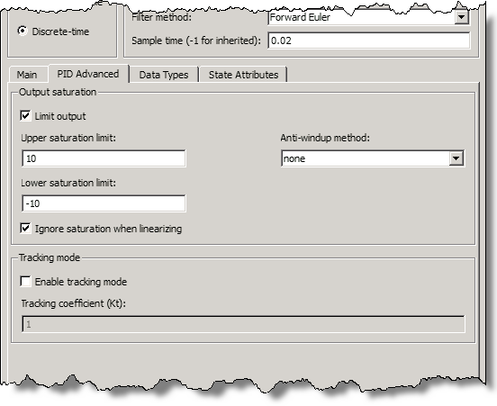
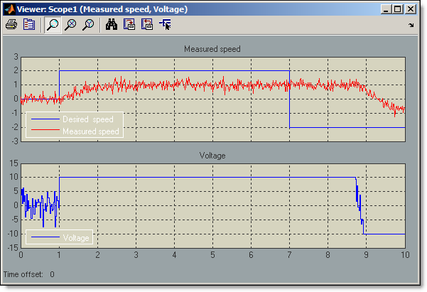
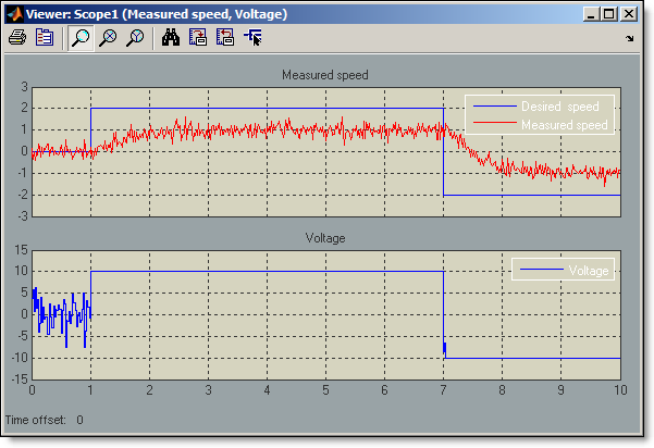
We see that at the time of the first step change at 1 second, voltage signal from the controller saturates at 10 Volts.  When desired speed drops at 7 seconds, the voltage does not decrease immediately and stays at 10 Volts for almost 2 more seconds.  This is the result of integrator wind-up in PID controller, which leads to undesired delay in tracking the speed command.  It can be fixed by enabling integrator anti-windup in the PID Controller block dialog. Rerunning the simulation with integrator anti-windup enabled, we see that the controller still cannot achive commanded speed value of 2 rpms –it simply does not have enough authority, but when the speed is commanded to -2 rpms, controller quickly responds to change in the requested speed.

As we saw, the new PID tuning method and the new PID Controller block helped us quickly tune our PID Controller, and create a discrete-time design that addresses output saturation and integrator wind-up issues.

Now it is your turn

Do you use PID control? How do you address integrator wind-up?  Leave a comment here and tell us how you tune your controller gains.

By Seth Popinchalk

15:00 UTC | Posted in Controls, Guest Blogger | Permalink | 16 Comments »

You can follow any responses to this entry through the RSS 2.0 feed. You can skip to the end and leave a response. Pinging is currently not allowed.

16 Responses to “PID Control Made Easy”

1. C.K. Wong replied on January 2nd, 2010 at 07:23 UTC :
   

   Hi,

   Thanks for the very useful tutorial. I’d like to know if the new PID block in Matlab can handle MISO system? What if my system model takes in 2 inputs?

   Best regards.

2. Arkadiy Turevskiy replied on January 4th, 2010 at 16:30 UTC :
   

   Hi C.K.,
   The PID Controller block by itself is a single input single output (SISO) block. For a MISO or MIMO system you can either break it into several SISO loops and design each one individually, or design a multivariable controller (such as LQR/LQG, H-infinity, model-predictive controller, etc).
   Arkadiy

3. Shahin Moghimi replied on February 8th, 2010 at 12:27 UTC :
   

   Hi,

   I have the R2008a version, and am wondering if there is such an automatic tool in my version as well for Simulink-based models PID tuning.

   Regards,
   Shahin

4. Guy replied on February 8th, 2010 at 14:18 UTC :
   

   @Shahin – The Simulink Control Design toolbox offers functionalities similar to the one provided by the new PID block, and more. An example can be found here:

   http://www.mathworks.com/access/helpdesk/help/toolbox/slcontrol/gs/brrqsnp.html

   Note that Simulink Control Design allows you to design PID controlers, but it can also help you tuning other types of more complex controllers.

   I also would like to mention the Simulink Design Optimization toolbox. If you have a plant which is very non-linear, sometimes tuning a controller with a linearized version of the plant is not appropriate. In that case Simulink Design Optimization runs an optimization algorithm directly on your Simulink model. An example can be found here:

   http://www.mathworks.com/access/helpdesk/help/toolbox/sldo/gs/brzts0c.html

   Note that in R2008a, this toolbox was named “Simulink Response Optimization”

5. ajinkya replied on April 1st, 2010 at 17:39 UTC :
   

   i have a project on dc motor speed control using pid .
   can you please send me the file(in simulink) u got this graphs from to my id ajinkyakhorgade@gmail.com
   i will be very thankfull to u

6. Arkadiy Turevskiy replied on April 1st, 2010 at 20:19 UTC :
   

   The model described in this post is available on MATLAB Central here:
   http://www.mathworks.com/matlabcentral/fileexchange/26275-pid-controller-design-for-a-dc-motor
   Enjoy.

7. Mac replied on September 6th, 2010 at 10:35 UTC :
   

   I want to use PID controller for quarter car model.

   will u help me in tuning the P I and D parameters for the controller?

8. misha replied on December 16th, 2010 at 19:39 UTC :
   

   Hii I just want to know how to tune PID controller from transfer function of the circuit. Unable to know how to change the PID parameters.

9. Arkadiy Turevskiy replied on April 27th, 2011 at 18:49 UTC :
   

   For a comprehensive collection of tutorials and demos on designing PID controller in MATLAB and Simulink, take a look at this page:
   PID Control with MATLAB and Simulink

10. Hendrick replied on September 3rd, 2011 at 13:08 UTC :
    

    Hi Arkadiy,

    I’m having difficulty tuning my controllers at the moment. My system consists of a PID controller feeding into a PI controller, I tuned the inner PI first but the values are always ridiculous…

    If I show you my .mdl, would you be able to tell me why it’s not autotuning?

    Thanks,

    Hendrick

11. Arkadiy Turevskiy replied on September 13th, 2011 at 16:52 UTC :
    

    Hi Hendrick,
    The PID Tuner highlighted in the post works on SISO loops. In case of a cascaded controller,like you have, you most likely need to open the outer loop, and tune the inner loop first. Then, with inner loop tuned, you can close the outer loop and tune it.
    This is explained in detail in this demo:
    http://www.mathworks.com/products/simcontrol/demos.html?file=/products/demos/shipping/slcontrol/scdairframectrldespad.html

    Another interesting point is that we actually just released a new capability to tune multi-loop or any multivariable control systems in Simulink, without changing controller structure.Take a look at these couple of demos:
    http://www.mathworks.com/products/demos/robust/tuning-decentralized-control-system-for-helicopter.html
    http://www.mathworks.com/products/robust/demos.html?file=/products/demos/shipping/robust/cascade_demo.html

    HTH.
    Arkadiy

12. Bassim Jassim replied on January 20th, 2012 at 07:44 UTC :
    

    Hi
    If the system has many loops i.e more than one controller. Is it possible to use this tool?

    many thanks

13. george replied on February 27th, 2012 at 17:06 UTC :
    

    Hello, I have a real model (Pendulum with a dc motor+propeller at the bottom and from RTW I controll the angle of the pendulum) and I want to use parametter estimation so I can find the real parameters! Could this work for the real model? I am a student. If you can help me! Thanks, George

14. Anand Vasappanavara replied on March 12th, 2013 at 09:30 UTC :
    

    I have worked on a chemical plant (Shell) control systems for over 5 years, unfortunately could not convince the top management for the introduction of Matlab and Simulink for Process Control (Tuning, System Identification, Process Optimization & Model Predictive control)in the industry. I want to know if any group is working to introduce these tools in the chemical industry, i would like to volunteer my time to help them.

15. syed replied on April 30th, 2013 at 15:58 UTC :
    

    Anand,

    I am trying to use these tools to help with making a PID autotuner using process data or online. It is a heater tank with very viscous flows.

16. sara replied on May 26th, 2013 at 06:30 UTC :
    

    hi
    i want design a pid controller for multivariable process?????????

Leave a Reply

<pre class="code">
a = magic(3);
sum(a)
</pre>

These postings are the author's and don't necessarily represent the opinions of MathWorks.