If you are attentive to details, you might have noticed that in MATLAB R2019b, we removed the First-Order Hold block from the Discrete section of the Simulink Library browser.

At the same time, we added in the Continuous section of the Simulink Library a new First Order Hold block.

Why a new First Order Hold?

One of the questions I receive the most often from Simulink users is: How can I speed up my model?

This new First Order Hold block has been designed especially to improve the performance of a common family of models: a continuous variable-step plant connected to a discrete controller.

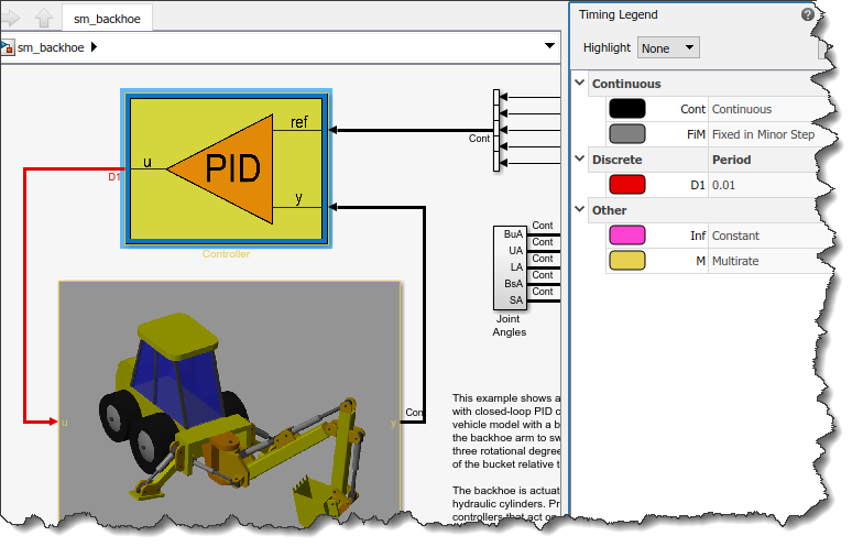
As an example, let's use the Backhoe example included with Simscape Multibody, where I discretized the controller to make it run at a 10 millisecond rate.

If I simulate this model through the Solver Profiler, I can observe that the model takes about 110 seconds to complete 60 seconds of simulation. This requires 16917 simulation steps, and most importantly, 6025 solver resets are being triggered along with 6214 Jacobian updates.

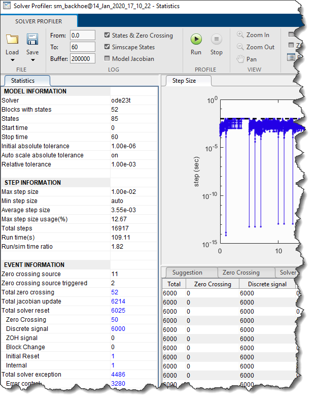
If you do the math, 60 seconds of a discrete rate at 0.01sec is 6000 steps. In Simulink, every time the value of a discrete signal driving a continuous plant changes, a solver reset is triggered. Depending on various criteria, a solver reset event can also trigger a Jacobian update - and Jacobian updates are an expensive operation, scaling exponentially with model size.

First Order Hold

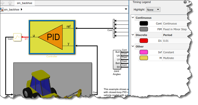
Let's try to insert the new First Order Hold block between the controller and the plant and rerun the solver profiler.

Now the simulation took only 16 seconds and most numbers are significantly down:

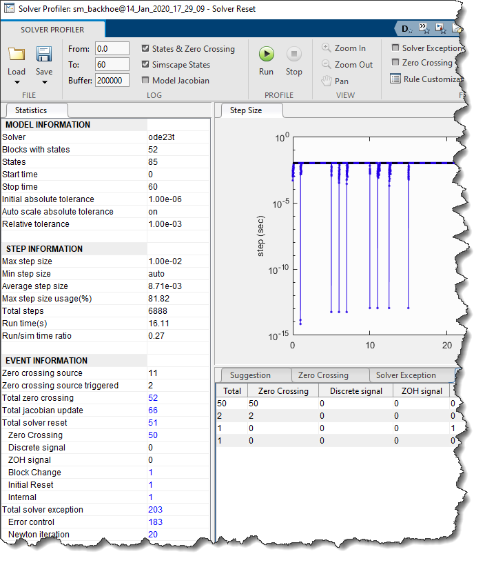
From 110 seconds to 16 seconds... That's a good speedup!

When to use the First Order Hold?

Now that you see such significant improvement, you might be wondering why we are not automatically applying this technique every time a discrete signal feeds continuous blocks. The reason is accuracy.

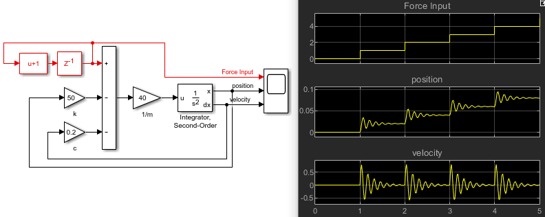
To illustrate the tradeoff you are making when introducing the new First Order Hold, let's use a simpler example. The following example is a simple mass-spring-damper system driven by a discrete ramp signal with a sample time of 1 second. As you can see, every time the input signal changes, it makes the mass-spring-damper system oscillate:

If we introduce the First Order Hold block, we can see that the results change significantly:

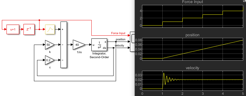
The reason is, as its name implies, the new First Order Hold block interpolates between the steps of the discrete rate to provide a continuous signal to the Integrator block. Here is a figure showing the signal before and after the block:

I will repeat it in bold: The new First Order Hold block can significantly speed up some simulations... but it can also impact the results. With great powers come great responsibilities :-)

To see if the First Order Hold can help you, try using the Solver Profiler. If you see a large amount of solver resets triggered by discrete signals, and those trigger Jacobian updates, the new First Order Hold block can probably speed up your simulation. After that, it is up to you to judge if the quantization effect introduced by the discrete rate affects the results significantly. If you are ok with how it impacts the results, you're good to go.

Now it's your turn

Give a try to the new continuous First Order Hold and let us know how it works for you in the comments below.