
Unifying MATLAB and Simulink: A User Story Part 4
In today's post, I continue extending the framework introduced over the past few weeks. If you missed the previous posts in this series, here are links:
- Unifying MATLAB and Simulink: A User Story Part 1: Parameterizing a model with MATLAB objects
- Unifying MATLAB and Simulink: A User Story Part 2: The slPart class, block template and data variants
- Unifying MATLAB and Simulink: A User Story Part 3: Controlling variants with MATLAB objects
- Unifying MATLAB and Simulink: A User Story Part 4: Post-processing and visualizing logged data
- Unifying MATLAB and Simulink: A User Story Part 5: Larger examples
So far in this series, the framework I introduced has been mostly focused on configuring a model, with the mindset of simply "picking a part" by instantiating a MATLAB object from a library of MATLAB classes. In this post, I extend the idea of "Unifying MATLAB and Simulink" to managing and post-processing logged data after simulation.
By the end, I hope you will see how this slPart framework leads to fully contained components that include pre-defined parameterizations, variants, and functions/methods to interact with it in MATLAB. Assuming the slPart has been created and validated by a domain expert, it can then be shared with other users and simply used in a straightforward and easy to discover manner.
A Method to Retrieve Logged Data
When I created the slPart class, I added a BlockPath property, mentioning that it was going to be useful later. It's now time to use it!
What I use BlockPath for is to retrieve the data logged inside the subsystem. For that, I create a method that takes a Simulink.SimulationOutput object and parses it to store the logged data in a newly added Log property of the slPart object. This method simply leverages the find method of the Simulink.SimulationData.Dataset object. Here is what the slPart class now looks like:
classdef slPart < handle
properties (Hidden = true)
BlockPath char
Log Simulink.SimulationData.Dataset
end
methods
function obj = maskInit(obj,blk)
% See previous posts
end
function obj = getLog(obj,out)
obj.Log = out.logsout.find('-regexp','BlockPath',[obj.BlockPath '(/.*)?$']);
end
end
end
That way, if I simulate a model with multiple parts, each part will be able to retrieve its own data.
For example, let's put two copies of the spring with variants created in the previous post and parameterize them with different objects.

Assign objects of different classes to each of them and simulate. Once the simulation is complete, each object can retrieve its own logged data:
mdl = 'spring_sim';
mySpring1 = springLib.springN1234;
mySpring2 = springLib.springNonLinearV1;
out = sim(mdl);
mySpring1.getLog(out);
mySpring2.getLog(out);
mySpring1.Log
mySpring2.Log
Defining Custom Post-Processing and Visualization
Now that each part is able to retrieve its own data, it becomes possible to define custom post-processing and visualization of the results for a part. To illustrate how this can work, I rearranged my example project a little bit to have both springLinear and springNonLinear subclassing the same spring superclass. Here is how the dependency of my classes now looks like in using the Class Diagram Viewer:
matlab.diagram.ClassViewer('Folders',currentProject().RootFolder);
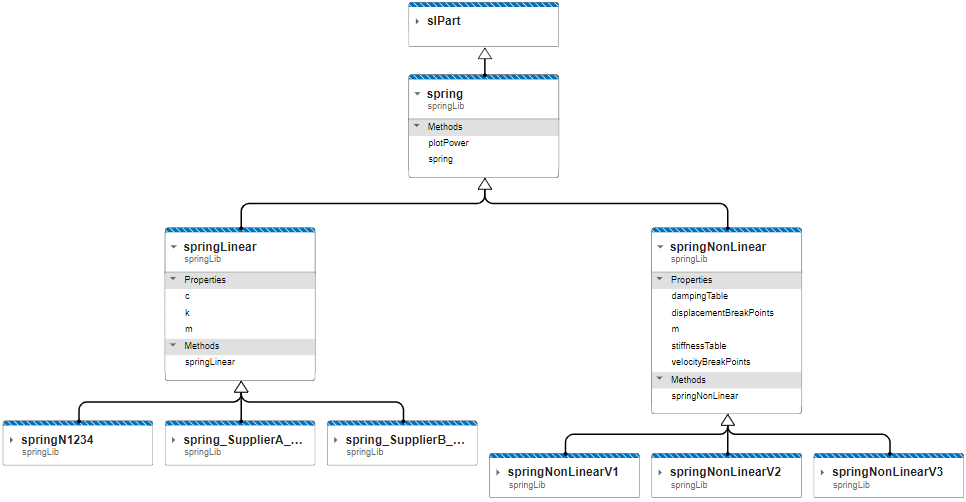
After this reorganization, I added a simple plotPower method to the spring class. Since each spring subsystem has two logged signals, named "velocity" and "force", I multiply them to create a "power" timeseries and plot it. Here is what the spring class looks like:
classdef spring < slPart
methods
function plotPower(obj)
power = obj.Log.get('velocity').Values*obj.Log.get('force').Values;
power.Name = 'Power';
plot(power)
end
end
end
Using the same model as above, I can then call this method for each object inheriting from the spring class.
mdl = 'spring_sim';
mySpring1 = springLib.springN1234;
mySpring2 = springLib.springNonLinearV1;
out = sim(mdl);
mySpring1.getLog(out);
mySpring2.getLog(out);
figure;
mySpring1.plotPower;
hold on
mySpring2.plotPower;

Now it's your Turn
Now that I covered variants and logging, I hope that the benefits of having a framework like this one are becoming clearer.
When sharing a component developed in this framework with other users, what they receive is not just an algorithm implemented in Simulink; they also receive a set of pre-defined parameterizations and a set of functions/methods to interact with it, created and validated by the domain expert who created the component.
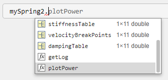
In addition to that, tab-completion also helps discovering what is available with such a component.
What you think of a framework like this one? Do you think future versions of Simulink should come with more built-in functionalities to facilite such a workflow? Let us know in the comments below.
- Category:
- Community,
- Masking,
- Modeling,
- Parameters


Comments
To leave a comment, please click here to sign in to your MathWorks Account or create a new one.