
Behavioral Models with Agentic-AI-powered MBSE

Today I am happy to welcome back Sarah Dagen from MathWorks Consulting Services for another visit to the Galactic Soup Factory!
.
When we left off using agentic AI and MBSE to design an intergalactic soup factory, we were evaluating 3 physical design variants. I am continuing the trade study in this article, but this time it is based on dynamic simulations rather than static analysis.

A reminder of what happened so far
I started by using a coding agent along with the Simulink Agentic Toolkit and System Composer to import and analyze system requirements and develop functional, logical, and physical architectures.
Then, I had the agent propose three different physical architecture variants that could meet the requirements, and developed architectural analysis and a trade study to evaluate the variants against each other.
These are our three architecture candidates:
HyperCook prioritizes throughput with four parallel continuous cook lines.

LeanBroth prioritizes budget margin with two batch kettles and one prep station.

EverSimmer prioritizes robustness: three fully independent production cells, each a complete prep-cook-quality control-pack chain. You can still produce soup even if one or two entire cells fail.
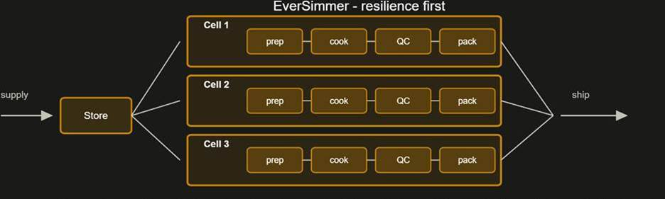
Using architectural analysis and trade study techniques, EverSimmer emerged a strong choice. It had the highest score in the majority of weighting scenarios.
Let’s add behaviors!
All of the analysis up to this point was based on static calculations and spec-sheet type data. To get a deeper understanding of how these different factories would actually work, I used the agent to help build some behavioral models. These are models that have executable semantics, like our static architectures, but also time-dependent equations.
When I originally designed these variants, I aimed to reuse as many architectural sub-components as possible. There are differences in peripheral details, but fundamentally they are all doing the same thing with different combinations of the same components – things like preparing ingredients, cooking, quality control and packaging. So when it came to modeling the behaviors, I asked the agent to create parameterized reference models that could be reused in all the architectures.
To start to get a feeling of how those factories operate, I worked with the agent and made the following component models:
Component model | What it models |
Storage | Storage buffer, starvation, and overflow |
Prep Unit | Preparation with rate limits and startup lag |
Cook Line | Continuous cooking and power consumption |
Cooking Vat | Batch cooking and thermal dynamics |
Quality Control Station | Inspection, contamination detection, and calibration |
Packager | Rate-limited packaging with backlog |
Production Supervisor | Production modes and failed-line control |
Production Cell | Integrated preparation through packaging |
I didn’t give the agent much direction on how to model anything. It made some technical decisions that I might not have made myself, but it generally got the job done and was good enough to bring insights. I told the agent to use the whole spectrum of modeling tools at its disposal. For example, for the cooking vat, the agent decided on its own to use Stateflow to implement the control mode logic and Simscape for the physical systems.
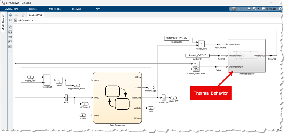
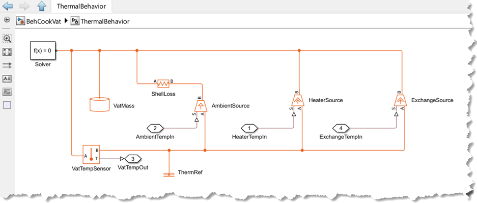
These are good choices, for a real project I would probably have spent more time planning with the agent before letting it build to make sure those decisions were my own.
The architecture is the model
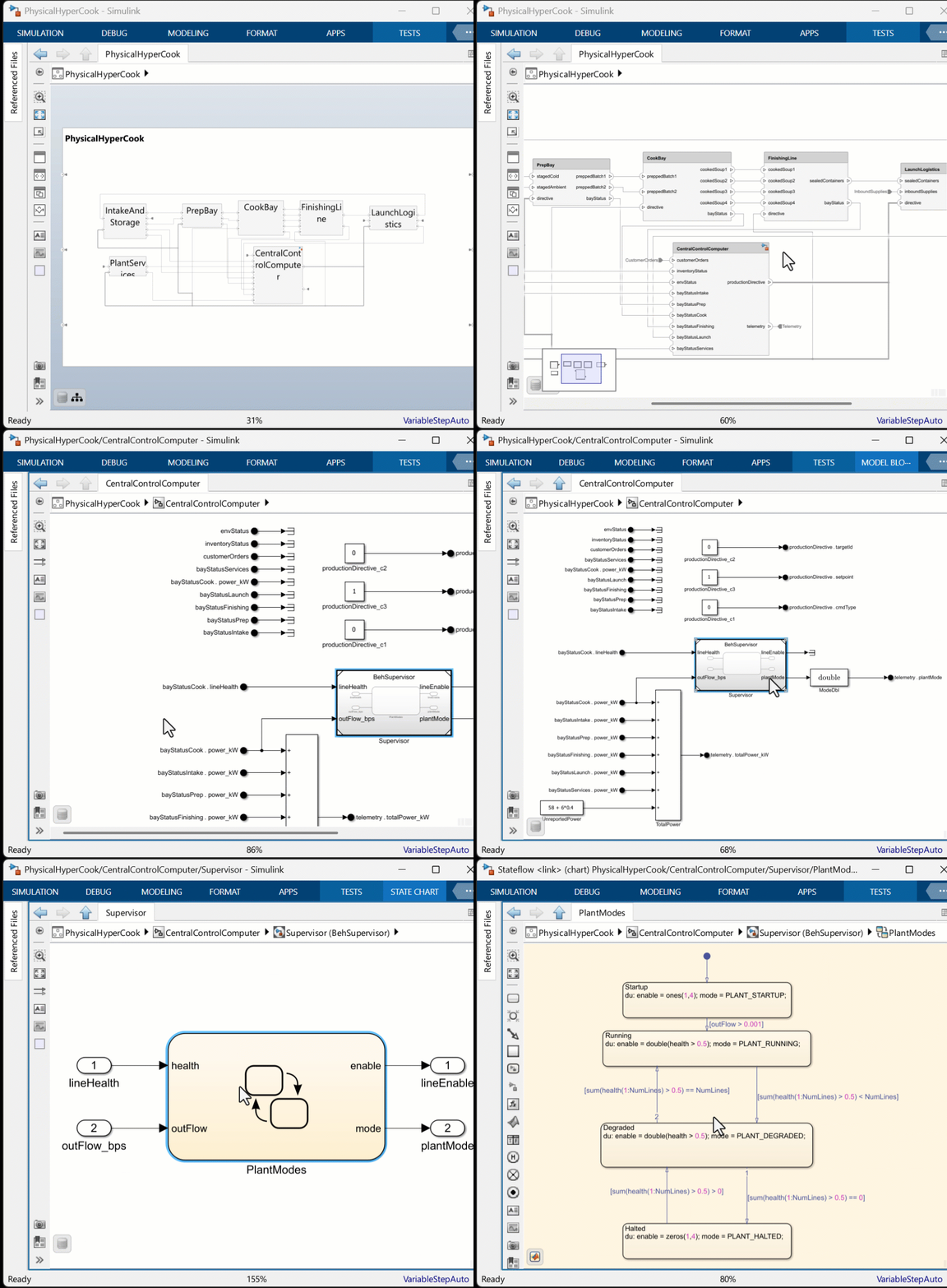
One of the most powerful features of System Composer is its simulation capabilities, which is very different from many other MBSE tools. You can add Simulink models and behaviors directly in System Composer architecture models!
Here’s a little video showing how you can navigate directly from a system-level architecture down into behavioral models – a state chart in Stateflow, in this case:
Simulating the dynamics
Once I had my architectures elaborated with behaviors, I needed to build simulation scenarios and test cases to observe the system dynamics.
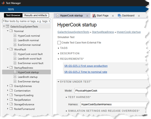
Working with the agent, I created several suites of tests to simulate different operational scenarios. The scenarios are based on the system requirements, and include traceability to the requirements.
Simulate!
Right away I can see interesting results. In the nominal operation case, I can see that the output of each factory varies over time even after it reaches nominal production, and sometimes has very large dips. Here’s the factory output rate of each variant from a cold start:
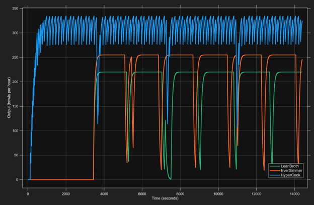
I wanted to dig in to what is causing the production rate changes, and I was especially interested in what is happening with LeanBroth at around 7,500 seconds.
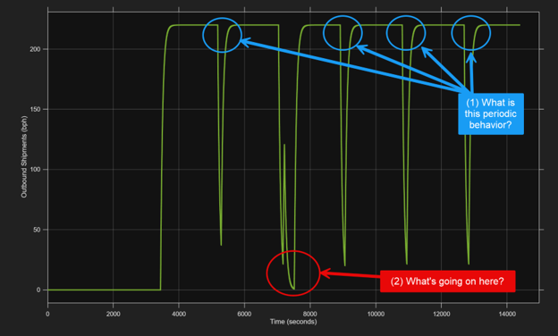
At first, I started doing what I would usually do: log signals I suspect are involved and start overplotting data until I find a relationship… but then I remembered: I have an agent! I asked that agent to explore the results and create plots that would explain the observations, and it came up with this:
First, the periodic dips in factory output:
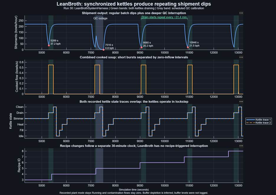
And next, what’s going on at around 7,500 seconds:
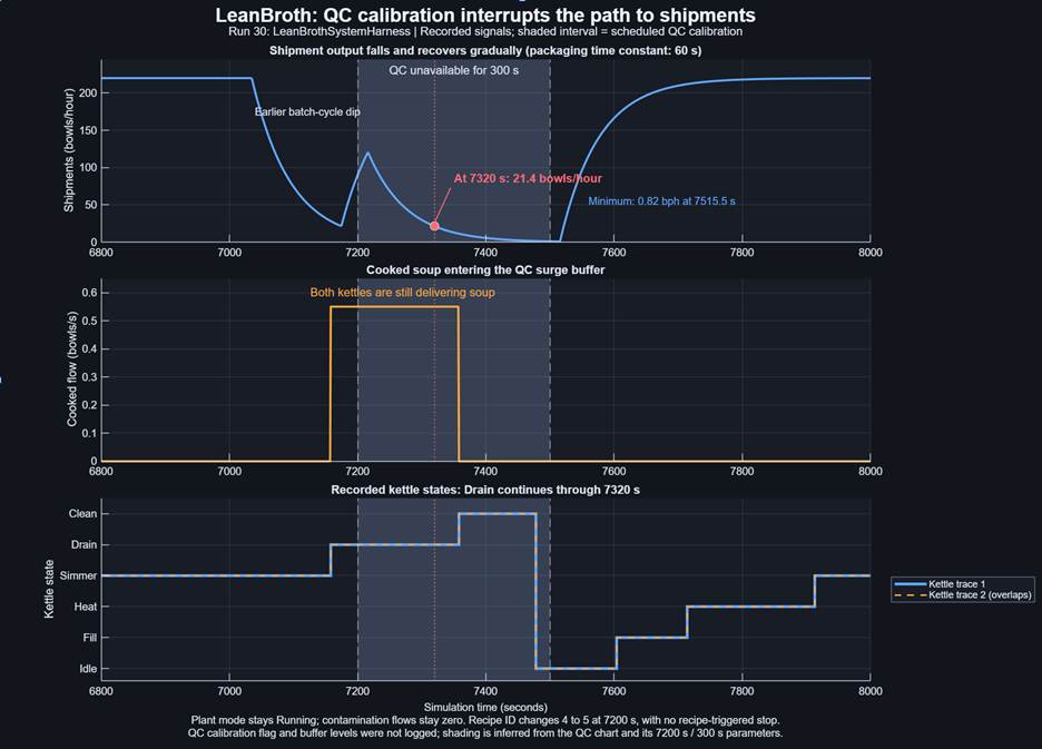
Those are interesting behaviors that I could only learn about with dynamic simulations, and it was very convenient to have the agent as a partner to investigate this.
System-level Insights
After running through different simulated operational scenarios, I was able to learn new things about my design variants. I asked the agent to summarize insights that were discovered after running both the static analyses and the dynamics simulations:
Observation | HyperCook | LeanBroth | EverSimmer |
Static → simulated throughput (bowls/hour) | 320 → 308.4 | 210 → 196.8 | 240 → 231.9 |
Time to first packaged output | 2.0 minutes | 57.3 minutes | 57.3 minutes |
Time to sustained nominal production | 13.6 minutes | 62.6 minutes | 62.6 minutes |
Energy per bowl (kWh) | 1.562 | 0.822 | 1.216 |
Production retained after worst single fault | ~ 0% | ~ 0% | 67.3% |
Summary
Adding behaviors brought the trade study beyond spec-sheet comparisons, revealing differences in operational behaviors including startup time, energy use, and fault resilience. The agent helped me build reusable models and explore these scenarios cheaply. Now, the choice of soup factory rests not just on its architecture, but on how it behaves in operation.
Now it's your turn
The whole project is on GitHub as a runnable reference example: models, requirements, analysis, tests, and the documentation set. You can open the project and open this guided tour.


评论
要发表评论,请点击 此处 登录到您的 MathWorks 帐户或创建一个新帐户。