Seth on Simulink

May 23rd, 2008

I remember while learning Simulink, drawing ordinary differential equations was one of the early challenges. Eventually I discovered a few steps that make it easier. First, rewrite the equations as a system of first order derivatives. Second, add integrators to your model, and label their inputs and outputs. Third, connect the terms of the equations to form the system.

Example: Mass-Spring-Damper

The mass-spring-damper system provides a nice example to illustrate these three steps. Let’s look at the equation for this system:

The position of the mass is , the velocity is , and the acceleration is .

Express the system as first order derivatives

To rewrite this as a system of first order derivatives, I want to substitute for , and for . Then I can identify my two states as position and velocity . The equation becomes

And this is rewritten at two first derivatives:

Velocity and position are the states of my system. When thinking about ODEs, states equal integrator blocks.

Add one integrator per state, label the input and output

I always make a point to write the equations as an annotation on my diagram. I refer to this as I add blocks to the canvas. Here are the two integrators for the mass-spring-damper system.

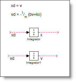
I draw signals from the ports and label inputs as the derivative (), and the output is the state variable.

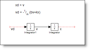
Connect the terms to form the system

The first connection is easy, , so I connect the output of the velocity integrator to the input of the position integrator. When this happens, aligning the integrators in the diagram shows that you have a second order system.

To implement the second equation, I add gains and sums to the diagram and link up the terms.

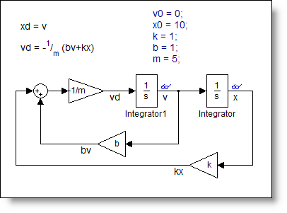
The final step, initial conditions

Modeling differential equations require initial conditions for the states in order to simulate. The initial states are set in the integrator blocks. Think of these as the initial value for v and x at time 0. The ODE solvers compute the derivatives at time zero using these initial conditions and then propagate the system forward in time. I used an annotation to record these initial conditions, v0 = 0, and x0 = 10.

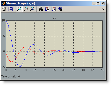
Simulating the model for 50 seconds produces the following trace for x (blue) and v (red).

Over time, I have become more comfortable in converting from equations to models, and I do not always rewrite the states. I think that fundamentally I still follow the same process:

1. Re-express the system in terms of state derivatives
2. Add integrators and label the inputs and outputs
3. Connect up the equations
4. Set initial conditions

Now it’s your turn

Is this the same process you learned when you started using Simulink? Do you have any special tips on how to draw ODEs? Share your ideas and leave a comment here.

19:46 UTC | Posted in Modeling, ODEs | Permalink |

You can follow any responses to this entry through the RSS 2.0 feed. You can skip to the end and leave a response. Pinging is currently not allowed.

10 Responses to “How to draw ODEs in Simulink”

1. Daniel replied on May 23rd, 2008 at 21:27 UTC :
   

   Hey Seth I’ve been trying to learn some Simulink and was glad MathWorks now has a Simulink blog!

   In relation to your post, what you recommend if my ‘kx’ is substituted with a ‘f(x)’ where we have non-linear stiffness. Currently I have it to substitute the gain block with a look up table. Are there other alternatives or suggestions? Should I be using the time varying transfer fcn blocks instead?

2. wei replied on May 27th, 2008 at 11:11 UTC :
   

   Hi Daniel,
   There are several choices from “user-defined functions” group of the Simulink library.

3. Wenting replied on May 30th, 2008 at 17:58 UTC :
   

   Hi Seth, I am trying to find a saddle path backwards from the equilibrium as it is very difficult for me to know the exact initial values on the saddle path for my four dimensional ODE system. I tried to use the code tspan=[T 0] instead of [0 T] (T could be any number) when I draw the graph.And I did not change the ODE system. The result turned out to be strange as it seemed that the system always stayed at the equilibrium point while it supposed to be a saddle point. My question is that do I need to add “-”(minus) in front of my ODE system as well? Or is there other advice? Many thanks!

4. Muralidhar M replied on July 16th, 2008 at 04:26 UTC :
   

   Hi Seth,

   The post on ODE was excellent…can we have a similar post on “Difference equations” and also on “partial differential equation”.

   Thanks!
   Murali

5. Mapa Ustka replied on August 6th, 2008 at 05:47 UTC :
   

   Nice Blog!Very good Blog!

6. RAMYA replied on August 29th, 2008 at 07:49 UTC :
   

   sir,
   am pursuing my masters in communication engineering. i am finding some difficult in implementing a block given in my paper, using simulink. Dynamic simulation of MEMS switches using Simulink® I VE ATTACHED THE PAPER FOR UR CONVENIENCE. PLEASE HELP ME IN IMPLEMENTING THE EQUATIONS AND BLOCKS IN SIMULINK. EXPECTING A POSITIVE REPLY FROM YOU AT THE EARLIEST SIR..
   D. J. Combes, K. M. Brunson and R. J. T. Bunyan
   QinetiQ Malvem, St Andrews Road, Malvem, Worcestershire, WR14 3PS
   ABSTRACT:
   A nodal model is implemented in Simulink and used to investigate the dynamics of electrostatically actuated MEMS switches. The model is based on reduced order 4DOF beam elements, with electrostatic forces based on simple parallel plate approximations at each node. Hard stops and contact stiction conditions are implemented. Using this model, the role of dynamic forces in overcoming contact stiction in MEMS switches is investigated. For an example MEMS switch, the relationship between the design of the switch, the strain energy under actuation and the dynamic restoring force are discussed. Dynamic forces are found to play a highly significant role in overcoming contact stiction.
   Keywords: MEMS switch, Simulink, Dynamic model, Stiction force
   GOD… AM UNABLE TO COPY THE BLOCK SETH…

7. Domek replied on October 17th, 2008 at 12:57 UTC :
   

   Great info!
   Will come handy one day. All students will be thankful.

8. Dujing replied on March 3rd, 2009 at 03:18 UTC :
   

   Thanks!It’s useful for me!

9. valio replied on August 26th, 2009 at 20:02 UTC :
   

   Hello Seth!

   I rebuild all as you advised:

   but it wasnt help to avoid problems:
   “Trouble solving algebraic loop..”
   as obvious on picture.

10. valio replied on August 26th, 2009 at 20:04 UTC :
    

    Hmmm..

    Here please: http://img220.imageshack.us/img220/5176/212d.jpg

Leave a Reply

<pre class="code">
a = magic(3);
sum(a)
</pre>

These postings are the author's and don't necessarily represent the opinions of The MathWorks.