Guy and Seth on Simulink

Contents

Embarrassingly Parallel Problems

PARFOR is the parallel for-loop construct in MATLAB. Using the Parallel Computing toolbox, you can start a local pool of MATLAB Workers, or connect to a cluster running the MATLAB Distributed Computing Server. Once connected, these PARFOR loops are automatically split from serial execution into parallel execution.

PARFOR enables parallelization of what are often referred to as embarrassingly parallel problems. Each iteration of the loop must be able to run independent of every other iteration of the loop. There can be no dependency of the variables in one loop on the results of a previous loop. Some examples of this in Simulink are problems where you need to perform a parameter sweep, or running simulations of a large number of models just to generate the data output for later analysis.

Computing the Basin of Attraction

To illustrate an embarrassingly parallel problem, I will look at computing the basin of attraction for a simple differential equation. (Thanks to my colleague Ned for giving me this example.)

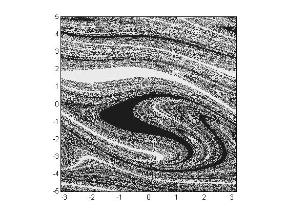
The equation is from an article about basins of attraction on Scholarpedia. When the system is integrated forward, the state will approach one of two attractors. Which attractor it approaches depends on the initial conditions of and its derivative, . The Scholarpedia article shows the following image as the fractal basin of attraction for this equation.

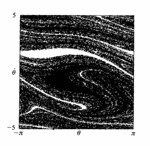
(picture made by H.E. Nusse)

Each of the thousands of pixels in that plot is the result of a simulation. So, to make that plot you need to run thousands of simulations.

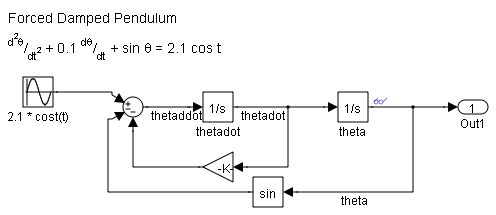
Forced Damped Pendulum Model

Here is my version of that differential equation in Simulink.

open_system('ForcedDampedPendulum')

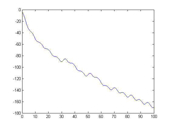
To see how evolves over time, here is a plot of 100 seconds of simulation. (Notice, I'm using the single output SIM command.)

simOut = sim('ForcedDampedPendulum','StopTime','100');
y = simOut.get('yout');
t = simOut.get('tout');
plot(t,y)
hold on

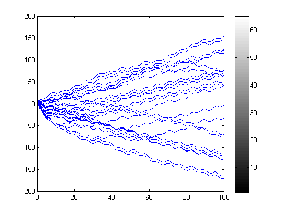
Nested FOR loops

Using nested for loops, we can sweep over a range of values for and . If we add that to the plot above, you can visualize the attractors at . I can use a grayscale colorbar to indicate the final value of at the end of the simulation to make a basin of attraction image.

n = 5;
thetaRange = linspace(-pi,pi,n);
thetadotRange = linspace(-5,5,n);
tic;
for i = 1:n
    for j = 1:n
        thetaX0 = thetaRange(i);
        thetadotX0 = thetadotRange(j);
        simOut = sim('ForcedDampedPendulum','StopTime','100');
        y = simOut.get('yout');
        t = simOut.get('tout');
        plot(t,y)
    end
end
t1 = toc;
colormap gray
colorbar

I have added TIC/TOC timing to the code to measure the time spent running these simulations, and from this we can figure out the time required per simulation.

t1PerSim = t1/n^2;
disp(['Time per simulation with nested FOR loops = ' num2str(t1PerSim)])

Time per simulation with nested FOR loops = 0.11862

During the loops, I iterate over each combination of values only once. This represents simulations that need to be run. Because the simulations are all independent of each other, this is a perfect candidate for distribution to parallel MATLABs.

Converting to a PARFOR loop

PARFOR loops can not be nested, so the iteration across the initial conditions needs to be rewritten as a single loop. For this problem I can re-imagine the output image as a grid of pixels. If I create a corresponding thetaX0 and thetadotX0 matrix, I will be able to loop over the elements in a PARFOR loop. An easy way to do this is with MESHGRID.

Another important change to the loop is using the ASSIGNIN function to set the initial values of the states. Within PARFOR, the 'base' workspace refers to the MATLAB workers, where the simulation is run.

n = 20;
[thetaMat,thetadotMat] = meshgrid(linspace(-pi,pi,n),linspace(-5,5,n));
map = zeros(n,n);
tic;
parfor i = 1:n^2
    assignin('base','thetaX0',thetaMat(i));
    assignin('base','thetadotX0',thetadotMat(i));
    simOut = sim('ForcedDampedPendulum','StopTime','100');
    y = simOut.get('yout');
    map(i)=y(end);
end
t2 = toc;

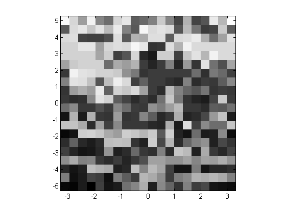
I can use a scaled image to display the basin of attraction. (Of course, this is verly low resolution.)

clf
imagesc([-pi,pi],[-5,5],map)
colormap(gray), axis xy square

The PARFOR loop acts as a normal for-loop when there are no MATLAB workers. We can see this from the timing analysis.

t2PerSim = t2/n^2;
disp(['Time per simulation with PARFOR loop = ' num2str(t2PerSim)])

Time per simulation with PARFOR loop = 0.13012

Local MATLAB Workers

Most computers today have multiple processors, or multi-core architectures. To take advantage of all the cores on this computer, I can use the MATLABPOOL command to start a local MATLAB pool of workers.

matlabpool open local
nWorkers3 = matlabpool('size');

Starting matlabpool using the 'local' configuration ... connected to 4 labs.

In order to remove any first time effects from my timing analysis, I can run commands using pctRunOnAll to load the model and simulate it.

pctRunOnAll('load_system(''ForcedDampedPendulum'')') % warm-up
pctRunOnAll('sim(''ForcedDampedPendulum'')')         % warm-up

Now, let's measure the PARFOR loop again, using the full power of all the cores on this computer.

n = 20;
[thetaMat,thetadotMat] = meshgrid(linspace(-pi,pi,n),linspace(-5,5,n));
map = zeros(n,n);
tic;
parfor i = 1:n^2
    assignin('base','thetaX0',thetaMat(i));
    assignin('base','thetadotX0',thetadotMat(i));
    simOut = sim('ForcedDampedPendulum','StopTime','100');
    y = simOut.get('yout');
    map(i)=y(end);
end
t3=toc;

t3PerSim = t3/n^2;
disp(['Time per simulation with PARFOR and ' num2str(nWorkers3) ...
    ' workers = ' num2str(t3PerSim)])
disp(['Speed up factor = ' num2str(t1PerSim/t3PerSim)])

Time per simulation with PARFOR and 4 workers = 0.025087
Speed up factor = 4.7285

Now that I am done with the local MATLAB Workers, I can issue a command to close them.

matlabpool close

Sending a stop signal to all the labs ... stopped.

Connecting to a Cluster

I am fortunate enough to have access to a small distributed computing cluster, configured with MATLAB Distributed Computing Server. The cluster consists of four, quad-core computers with 6 GB of memory. It is configured to start one MATLAB worker for each core, giving a 16 node cluster. I can repeat my timing experiments here.

matlabpool open Cluster16
nWorkers4 = matlabpool('size');
pctRunOnAll('load_system(''ForcedDampedPendulum'')') % warm-up
pctRunOnAll('sim(''ForcedDampedPendulum'')')         % warm-up

Starting matlabpool using the 'Cluster16' configuration ... connected to 16 labs.

n = 20;
[thetaMat,thetadotMat] = meshgrid(linspace(-pi,pi,n),linspace(-5,5,n));
map = zeros(n,n);
tic;
parfor i = 1:n^2
    assignin('base','thetaX0',thetaMat(i));
    assignin('base','thetadotX0',thetadotMat(i));
    simOut = sim('ForcedDampedPendulum','StopTime','100');
    y = simOut.get('yout');
    map(i)=y(end);
end
t4 = toc;

t4PerSim = t4/n^2;
disp(['Time per simulation with PARFOR and ' num2str(nWorkers4) ...
    ' workers = ' num2str(t4PerSim)])
disp(['Speed up factor = ' num2str(t1PerSim/t4PerSim)])

Time per simulation with PARFOR and 16 workers = 0.0064637
Speed up factor = 18.3521

matlabpool close

Sending a stop signal to all the labs ... stopped.

Timing Summary

Here is a summary of the timing measurements:

disp(['Time per simulation with nested FOR loops = ' num2str(t1PerSim)])
disp(['Time per simulation with PARFOR loop = ' num2str(t2PerSim)])
disp(['Time per simulation with PARFOR and ' num2str(nWorkers3) ...
    ' workers = ' num2str(t3PerSim)])
disp(['Speed up factor for ' num2str(nWorkers3) ...
    ' local workers = ' num2str(t1PerSim/t3PerSim)])
disp(['Time per simulation with PARFOR and ' num2str(nWorkers4) ...
    ' workers = ' num2str(t4PerSim)])
disp(['Speed up factor for ' num2str(nWorkers4) ...
    ' workers on the cluster = ' num2str(t1PerSim/t4PerSim)])

Time per simulation with nested FOR loops = 0.11862
Time per simulation with PARFOR loop = 0.13012
Time per simulation with PARFOR and 4 workers = 0.025087
Speed up factor for 4 local workers = 4.7285
Time per simulation with PARFOR and 16 workers = 0.0064637
Speed up factor for 16 workers on the cluster = 18.3521

A Quarter Million Simulations

Many months ago I tinkered with this problem, using a high performance desktop machine with 4 local workers, and generated the following graph. This represents 250,000 simulations.

Performance Increase

There are many factors that contribute to the performance of parallel code execution. Breaking up the loop and distributing it across workers represents some amount of overhead. For some, smaller problems with a small number of workers, this overhead can swamp the problem. Another major factor to consider is data transfer and network speed; transferring large amounts of data adds overhead that doesn't normally exist in MATLAB.

Now it's your turn

Do you have a problem that could benefit from a PARFOR loop and a cluster of MATLAB Workers? Leave a comment here and tell us all about it.

Get the MATLAB code

Published with MATLAB® 7.11