
THE Most Useful Command for Debugging Variable Step Solver Performance
Today I want to share a trick I often use to determine if a variable step simulation runs as fast as it should.
Visualizing the steps taken by a model
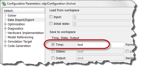
To begin, save the simulation time data. This can be done from the Data Import/Outport pane of the model configuration.
Once the simulation is completed, plot the derivative of the time data. This can be done with the following line:
semilogy(tout(1:end-1),diff(tout))
I like to use a logarithmic scale for the Y-axis because the time steps taken can vary over a very large range.
Now let's look at a few examples showing what kind of information we can extract from this figure.
Tolerance Exceeded
When applying this technique to the example demo vdp.mdl, we obtain the following figure:
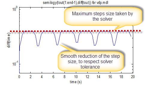
Using this figure, we can identify 2 main things.
First, we can see that most of the time, the steps taken by the solver correspond to the max step size specified in the model configuration. This means that you might be able to increase solver max step size and allow the solver to take larger steps, reducing the total number of steps needed to finish the simulation.
Secondly, we see that at some instants, the time steps reduces smoothly. This means that the solver takes steps as large as possible to respect the specified tolerance.
To confirm the above, let's change the solver max step size and see how it affects the step size:
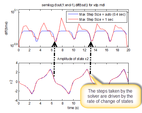
In this example, the effect is pretty small. But we can see that if we increase the max step size, the simulation takes larger steps.
Note that I recommend being cautious when increasing the solver max step size or tolerances. Take the time to do a convergence study to ensure the results still provide the accuracy you need.
Zero-Crossing
Another important pattern that can be identified using this technique is the effect of zero-crossings on the simulation.
Let's take this simple model, made of a sine wave connected to a saturation block.
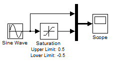
In this example, the Saturation block generates a zero-crossing event every time it enters or exits saturation. As we can see, this forces the Simulink solver to take very small steps to accurately capture this event.
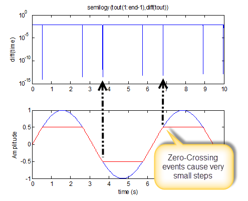
The zero-crossing mechanism provides accuracy by taking small steps. Knowing that is the behavior of the solver, it is up to you to judge if a block needs zero-crossing or not.
Conclusion
If your model runs slower than you expect, this technique can help you determine if it is because it takes smaller steps than it needs to.
In my debugging toolbox, this is one of the first things I try when I am investigating the performance of a simulation.
Now it's your turn
Do you have any tricks to share to help determinining if a variable-step simulation runs as fast as it can? Please share it by leaving a comment here.
- Category:
- Analysis,
- Numerics,
- ODEs,
- Performance,
- Simulation,
- Simulink Tips


Comments
To leave a comment, please click here to sign in to your MathWorks Account or create a new one.