
Optimizing the Hyperloop Trajectory
This week, Matt Brauer is back to describe further analysis of the hyperloop transportation concept.
The world is not flat
We previously published two-dimensional analysis for deriving a route for the hyperloop based on lateral acceleration limits. This time I looked at the other dimension of the problem: Elevation. This will complete the input data needed to fully simulate the Hyperloop.
I used optimization to determine the best elevation profile, combining pillars and tunnels along the route. I ended up with about 86 km of tunnels, with the longest continuous tunnel being about 2 km long. This result is about three times the amount of tunneling indicated in the alpha design document. Of course, this conclusion is heavily influenced by the approach used to optimize pillar height and vertical g-forces.
 Derived elevation profile for the hyperloop
Here’s how I came to my results.
Assumptions and Formulation
I started with the assumption that the 2-D route is fixed. This assumption makes elevation a 1-D problem, which is simpler than tackling three dimensions simultaneously. However, the problem is still non-trivial. I decided to use the Optimization Toolbox for the heavy lifting.
In my experience, there are four critical elements that guide successful use of optimization techniques:
- Formulation of the data
- Cost function
- Optimization routine configuration
- Initial Guess
The right combination of these elements can be very effective at solving complex problems. I’ll describe briefly how I set these elements to solve this problem.
Data to be optimized
I chose a simple formulation for the optimization data. I used a vector of pillar heights/depths spaced every 30m along the route. I found that to keep the optimization problem manageable I needed to break up the route into 12 sub-sections. The convergence time seemed to rise asymptotically with larger data sets.
Defining the cost function
To perform a numeric optimization, there must be a quantified evaluation of the solution. This cost function can then be minimized using the Optimization Toolbox to converge on the best solution. I chose to incorporate two elements into the cost function; (1) construction costs due to height/depth of the tube and (2) passenger comfort based on vertical acceleration. I created the tables below to quantify these cost elements at each point along the route.
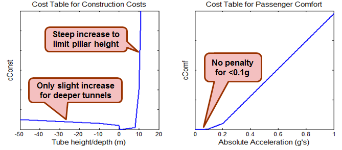 Cost tables for Construction Costs and Passenger Comfort
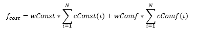
The equation below is used to arrive at a final value for the complete route. I can influence the relative priority of passenger comfort and construction costs by adjusting wConst and wComf.
Configuring the Optimization Routine
To calculate the cost function on the optimization data, I needed additional data such as ground elevation. I was able to pass these data to my cost function elevOpt by creating the function handle below. This statement defines x as the optimization data, but allows z_dist (translational distance), z_elev (ground elevation) and z_vel (vehicle velocity) to be passed as arguments as well.
% Create function handle for passing additional data
handle_trajOpt  = @(x)elevOpt(x,z_dist,z_elev,z_vel);
I tried several different optimization algorithms and found the best results using the quasi-newton algorithm of fminunc. I also had to increase the maximum iterations and function evaluations to ensure that I reached an adequate solution.
% Set options
options     = optimoptions(@fminunc,'Algorithm','quasi-newton',...
            'Display','iter','MaxIter',5000,'PlotFcns',{@optimplotfval,@plotElevOpt},...
            'MaxFunEvals',1e7);
The initial guess
I started my investigation trying two different starting points; a constant 3m height above the ground and an absolutely flat trajectory with constant elevation. It was interesting how the initial guess for the trajectory would affect the speed of the optimization and the final result. I was able to visualize how the results were shaping up with a customized plotting function. You can see in the code above how that function, plotElevOpt, was passed as a PlotFcns parameter in the optimization options.
Here are two examples with the uniform and flat seeds. To keep them interesting, these plots have been sped up about 5x.
[x, ~, ~, ~ ] = fminunc(handle_trajOpt,x0,options);
Here is the evolution of the optimization starting with a constant 3m height above the ground:
 Optimization with uniform height initial guess
And now starting with a flat constant elevation:
 Optimization with flat initial guess
For several of the route sections, a hybrid of the two worked best. I ended up using the fit function from the Curve Fitting Toolbox on the constant height trajectory to start with a smoother curve as initial guess. This profile generally followed the ground elevation but didn't have the excessive vertical acceleration peaks. For flatter sections, this initial guess came very close to the final solution.
Now it’s your turn
How would you approach identifying the optimal Hyperloop route? Let us know by leaving a comment here.


Comments
To leave a comment, please click here to sign in to your MathWorks Account or create a new one.