
Simulink Debugger: Monitoring Variable Step Solver Performance
A few months ago I introduced my favorite command to analyze the performance of a variable-step solver.
This week, I will introduce how the Simulink Debugger can be used for a deeper analysis of variable-step solvers performance. For this, we will use the debugger command-line interface.
Launching the debugger
For this example, let's use the demo model vdp.mdl. I start the debugger using sldebug and enable tracing of the solver information using strace 1. For this example, I want to run just a small part of the simulation, so I will set a breakpoint after 5 seconds using tbreak 5.

After using the continue command (or the one-character shortcut c), a lot of information is displayed.
Solver Information
Let's look at a successful step where we moved from 0.284s to 0.54s.
 (click to view full size)
In the above screen capture, you can identify:
- TM: We take a major step at 0.284s
- Tm - Hm: We start a minor step at 0.284s. Based on the evolution of the states during the previous step, the solver thinks this minor step should advance by 0.256 seconds.
- Tm - H: Nothing is blocking us from trying this step, we begin the integration from 0.284s and advance by 0.256s
- Ts - Hs: The minor step was successful, we move forward by 0.256s without exceeding solver tolerance
- Err - Ix: Among all the states in the model, the one closest to the maximum tolerance was state 1 and it's normalized error was 8.2045e-2. The normalization is made relative to the maximum tolerance. An error above 1 exceeds the tolerance and below one passes.
For more details on how to interpret the solver trace information, you can look at the documentation for strace.
To determine which state had the maximum error, use the states command:
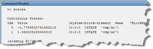
For this step, the state closest to the maximum tolerance (Ix=1) is from the Integrator block x2.
Step limited by maximum step size
Now let's look at a different type of output. If we move forward to 4.651s, we notice a step where the step size is limited by the solver maximum step size:
 (click to view full size)
If you see many of those in your model, this probably means you could increase the maximum step size in the solver configuration.
Failed step
Of course, not all steps move forward smoothly. Sometimes the solver needs to take steps back to respect tolerances. If we continue to step forward, at t=13.21s we notice that it took 2 attempts before respecting the tolerance. (click to view full size)
If this happens often in your model, you might want to try other solvers, like stiff solvers. If this does not help, you might want to look at your equations and the block with the maximum error.
Conclusion
The examples I have given show how the Simulink debugger can be useful to understand why a variable-step solver takes steps of a certain size. Those examples are mainly focused on states, but you can follow the same principle for zero-crossings by using functions like zcbreak and zclist.
I need to stop here because this post is already long enough, but I want to mention that those examples are only the tip of the iceberg. With the Simulink debugger, it is possible to see finer details of the integration done during minor steps and display data for any signal or block.
Now it's your turn
Take the time to go through the list of Simulink debugger Commands and let us know if you find something you will use by leaving a comment here
- Category:
- Debugging,
- Numerics,
- ODEs


Comments
To leave a comment, please click here to sign in to your MathWorks Account or create a new one.